Transcription of Excel Tables & PivotTables - Colorado State University
1 Excel PivotTables 1 Technology Training Center Colorado State University Excel Tables & PivotTables A PivotTable is a tool that is used to summarize and reorganize data from an Excel spreadsheet. PivotTables are very useful where there is a lot of data that to analyze. PivotTables are dynamic, meaning the data can be reorganized and redisplayed easily based on what the end result is to be. Even though PivotTables are dynamic, it is best to plan out the end result for the data, before creating a PivotTable. It is best practice to format the data as a table before creating a PivotTable because if data is ever added to or deleted from the original data, a table will automatically adjust to allow for the newly added, or deleted data to be displayed in the PivotTable, as long as the PivotTable data is refreshed. Tables Tables are very beneficial when working with large amounts of data, especially if that data may potentially change.
2 Tables give a nice visual layout of the data so it is easier to search out individual rows, sort and/or filter the data. Benefits of using Tables : Integrated Filter and Sort functionality Header row remains visible while scrolling, as long as the cursor is within the Table Automatic expansion and subtraction of the table when new data is entered Automatic adjustment charts when new data is entered Automatic reformatting of the table when new data is entered To convert a block of data into a Table, place the cursor within the data. Navigate to the Insert Tab and then click on the Table icon. Excel will populate the Format As Table dialog box, which will confirm the location of the data to be converted into a table, as well as an option to specify if the data contains headers. When the data location and the header option is selected, click OK. Excel PivotTables 2 Technology Training Center Colorado State University The look of the data on the sheet will change slightly, with the addition of a more distinct header row, alternating colored rows, as well as with filtering/sorting options applied to each heading.
3 If any columns of the original data have formatting applied, that formatting will carry over to the data within the table. Table Sizing Handle On the lower right corner of the table, there is a dark icon, called the Sizing Handle. The sizing handle indicates the bottom, right side of a table. Table Tools Any time the cursor is within the table data, the Table Tools Design Tab will be displayed on the right side of the ribbon. To make any changes to a table, the cursor must be located within the table data. To change the color scheme of a Table, make sure the cursor is within the table and then navigate to the Table Tools Design Tab. On the right hand side of the Design Tab is the Table Styles group. To select a new color, simply click on the color option to apply it to the table. To view more options than what are displayed, click on the dropdown menu on the lower right corner of the Table Styles group. Excel PivotTables 3 Technology Training Center Colorado State University Create a PivotTable When creating a PivotTable, it is best practice to ensure the data does not contain subtotals or blank cells.
4 Blank data may cause issues within the PivotTable by creating column names or cells to display as (blank). Tip: It is best practice to convert the data into a table before creating the PivotTable. Recommended PivotTables Recommended PivotTables is a feature introduced to Excel 2013 which provides a few PivotTable options based on the data in a worksheet. To use the Recommended PivotTables feature, make sure the cursor is within the data. Navigate to the Insert tab, and then select the Recommended PivotTables icon. A new Recommended PivotTable window will appear showing the options that Excel is recommending for the PivotTable. Users are able to click on each option to see a preview of how the PivotTable will display. Recommended PivotTables can be a useful option to use for a starting point for a PivotTable, but it may not be the best option based on what is expected as an end result. If none of the options are going to work, click on the Blank PivotTable button to create a Blank PivotTable button on the lower left side of the Recommended PivotTables window to create a blank PivotTable.
5 Tip: To view PivotTable Recommendations on an existing PivotTable, make sure the cursor is within the PivotTable. Navigate to the PivotTable Tools Analyze Tab and then click on the Recommended PivotTables icon. Note: To make changes to a PivotTable, the PivotTable Tools tab must be active. If the PivotTable Tools tab is not active, move the cursor within the PivotTable. Excel PivotTables 4 Technology Training Center Colorado State University Manual PivotTable To create a manual PivotTable, make sure the cursor is within the table (data) on the worksheet. Navigate to the Insert Tab and then click on the PivotTable icon. Note: Users may also select the data on the worksheet, navigate to the Insert tab, and then click the PivotTable icon. On the Create PivotTable window, make sure the correct table, or data range, is selected in the Select a Table/Range textbox. If the range is incorrect, move the cursor into the Select a table or range textbox and then highlight the correct data from the sheet.
6 On the bottom of the Create PivotTable window, choose the location to place the PivotTable, either a new worksheet, which will be automatically created to the left of the current sheet, or an Existing Worksheet. If the Existing Worksheet option is selected, click within the Location textbox and then navigation to the sheet and cell location to insert the PivotTable. When all of the options have been selected, click on the OK button to create the PivotTable Excel PivotTables 5 Technology Training Center Colorado State University The PivotTable will be inserted onto a sheet and will look similar to the screenshot below. The PivotTable consists of a blank PivotTable on the left side of the screen, the PivotTable Fields (column headings from the original data), on the top, right side of the screen, and the PivotTable areas on the bottom right side of the screen Note: To make changes to a PivotTable, the PivotTable Tools tab must be active.
7 If the PivotTable Tools tab is not active, move the cursor within the PivotTable. Excel PivotTables 6 Technology Training Center Colorado State University Add Fields to a PivotTable To make a PivotTable, fields must be added to the PivotTable areas. To automatically add a field to a PivotTable, click on the checkbox next to the Field name and Excel will place the field in the area that it sees is the best fit for that field. Note: This can be a good way to start working with PivotTables , but typically a manual process is a better option for adding fields to a PivotTable To manually add a field, click and hold on a field name and then drag the name into one of the four PivotTable areas listed below the field list. If the PivotTable isn t displaying the information as intended, users are able to drag fields into any of the other field areas on the fly by clicking and holding on a Field, and then dragging the field name into a new area.
8 Tip: Not every field has to be used when creating a PivotTable, there may be times when only 2 or three fields are used, and there may be times when all fields are used. This is a major benefit of PivotTables , they are dynamic so there is no right answer, it all depends on what information is to be displayed. PivotTable areas 1. Filters Top-level filters that are displayed above the PivotTable a. Filters can be used to only display results that meet a certain criteria i. For example, only display results for a single region vs all regions 2. Columns Display as column labels across the top of the PivotTable, with the data displayed below. Field names on the top of the columns area will display on the top within the PivotTable. Columns may have several fields added to them to nest the column labels. Single Field within Columns Excel PivotTables 7 Technology Training Center Colorado State University Nested fields within Columns 3.
9 Rows Display as row labels on the left side of the PivotTable. Rows may also have several fields to nest the row labels. Single field within Rows Nested fields with Rows 4. Values Displays as a calculation of the data in the field. The calculation can be a sum, count, average, etc. Excel PivotTables 8 Technology Training Center Colorado State University Remove Fields from a PivotTable To remove a field from a PivotTable, uncheck the field name from the Choose fields to add to report area section of the PivotTable Fields, or click, hold and drag the field name from the areas section back into the Fields section. Changing the Data Source If data is added to the PivotTable source data, and if the PivotTable was created without using a table, a new data source may have to be selected to ensure the PivotTable contains the newly added data. To change the original data source, make sure the cursor is within the PivotTable, navigate to the PivotTable Tools Analyze tab and then click on the Change Data Source button.
10 Select the new data range from a, which may be on a different worksheet, or workbook and then click on the OK button. Tip: The Change Data Source option may also be used to verify where the original data is located. Note: If the new data is coming from an external data source, a new PivotTable will have to be created and the option for External Data Source will have to be selected in the Create PivotTable dialog box. Excel PivotTables 9 Technology Training Center Colorado State University Delete a PivotTable from a Worksheet To delete, or clear all of the data from, a PivotTable make sure the cursor is in a cell in the PivotTable. Navigate to the PivotTable Tools Analyze tab, in the Actions group, click on the Clear button, and select the Clear All option. Another way to clear data from a PivotTable would be to deselect all of the fields in the PivotTable task pane. PivotTable Options The settings for how a PivotTable will display by default are located PivotTable options menu.