FACTORIZATION of MATRICES - University of Texas at Austin

1 FACTORIZATION of MATRICES Let's begin by looking at various decompositions of MATRICES , see also Matrix FACTORIZATION . In CS, thesedecompositions are used to implement efficient matrix algorithms. Indeed, as Lay says in his book: "In the language of computer science, the expression of as a product amounts to a pre-processing ofthe data in , organizing that data into two or more parts whose structures are more useful in some way,perhaps more accessible for computation."Nonetheless, the origin of these factorizations lies long in the past when they were first introduced by variousmathematicians after whom they are frequently named (though not always, and not always chronologicallyaccurately, either!). Their importance in math, science, engineering and economics quite generally cannot beover-stated, however. As Strang in his book says: "many key ideas of linear algebra, when you look at them closely, are really factorizations of a original matrix becomes the product of 2 or 3 special MATRICES .

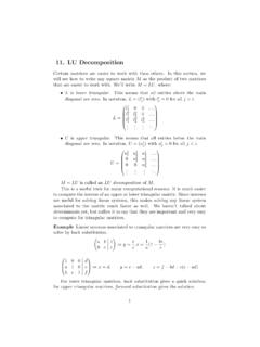
2 " But FACTORIZATION is really what you've done for a long time in different contexts. For example, eachpositive integer , say , can be factored as a product of prime integers, while eachpolynomial such as can factored as a product of linearfactors with real roots and a quadratic factor for which no further FACTORIZATION can be carried out. In thislecture we shall look at the first of these matrix factorizations - the so-called LU-Decomposition and itsrefinement the LDU-Decomposition - where the basic factors are the elementary MATRICES of the last lectureand the FACTORIZATION stops at the reduced row echelon form. Let's start. Some simple hand calculations show that for each matrix Gauss Decomposition:Notice that in the -term FACTORIZATION the first and third factors are triangular MATRICES with 's along thediagonal, the first (ower) the third (pper), while the middle factor is a (iagonal) matrix. This is anexample of the so-called -decomposition of a matrix.

3 On the other hand, in the term -factorizationboth factors are triangular MATRICES the first ower and the second pper, but now the second one allowsdiagonal entries which need not be . It is an example of the important -decomposition of a matrix. As weshall see shortly, this decomposition - possibly the most important FACTORIZATION of all - comes from themethod of elimination for solving systems of linear 2332P(x)= 16x4P(x)=(x 2)(x+2)(+4)x22 2[] = [][][] = [][],a bca10ba11ca01a0bad bca31 LUDLDU2LU1LU But what information might we get from such decompositions? Well, note the particular factors occuring inthe Gauss Decomposition of a matrix: if , then each factor is an elementary matrix as defined in the previous lecture, and soinvertible. In fact, by the known inverses given in Lecture 06,On the other hand, . Thus by Gauss Decomposition,as a matrix product calculation shows. Why bother? We knew this already from a simple direct calculation!

4 That's the point: except for the ,there's no formula for computing the inverse of a general matrix. But if we can decompose a generalmatrix into simpler components, each of which we know how to invert, then can be calculated interms of a product just as we've just showed using the Gauss Decomposition. What's more, as in the case where the condition was needed for the diagonal matrix to be inverted, use of adecomposition often shows what conditions need to be imposed for to exist. As we saw in Lecture 05, each of the elementary MATRICES in the Gauss Decompositiondetermines a particularly special geometric transformation of the plane: in the -term FACTORIZATION , the lowerand upper triangular MATRICES correspond to shearing the -plane in the and -directions, while thediagonal matrix provides a stretching of the plane away from, or towards, the origin (dilation).But without the Gauss Decomposition, would you have guessed that every invertible matrix determinesa transformation of the plane that can be written as the composition of shearings and dilation provided ?

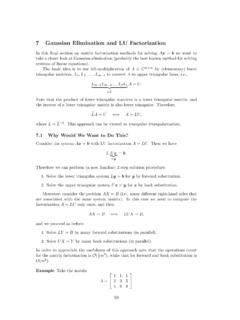
5 To handle the case when and , interchange rows by writing:Do the calculation to see why the lower triangular matrix didn't appear! Notice that the first matrix in thisdecomposition is again an elementary matrix - the one interchanging row 1 and row 2. As a geometrictransformation it reflects the -plane in the line . So both of the previous interpretations still applywhether or . What happens, however, if ? Well, cannot be reduced to echelon form! This suggests2 2ad bc 0 = [], = [], = [].[]1ca01 11 ca01[]a00ad bca 11a00aad bc[]10ba1 110 ba1(AB=) 1B 1A 1 = [][][] = ,[]acbd 110 ba11a00aad bc1 ca01 dad bc cad bc bad bcaad bc 2 2n nAA 12 2ad bc 0A 12 23xyyx2 2a 0a=0c 0[] = [][] = [][][].0cbd0110c0db0110c00b10dc1xyy=xa=0 a 0a,c=0[]00bdhypotheses for general results: Fundamental Theorem 1: if an matrix can be reduced to row echelon form without rowinterchanges, then has an -decomposition where is lower triangular with entries on thediagonal and is upper triangular.

6 Fundamental Theorem 2: if an matrix can be reduced to row echelon form possibly withrow interchanges, then has an -decomposition where is a product of row interchangeelementary MATRICES , is lower triangular with entries on the diagonal and is upper triangular. Fundamental Theorem 2 is the version that's most often used in large scale computations. But rather thanprove the existence of either decomposition in generality, let's concentrate on using a given decomposition insolving a system of linear 1: solve the equation whenand has an -decomposition Solution: set . Then and so . Now by the known inverse of lower triangular MATRICES given in lecture06,in which case the equation reduces toBut thenBecause is in upper triangular form this lastequation can be solved in several different example, the associated augmented matrixis in echelon form, so the solutions can be read offby back substitution as we did earlier in lecture01: Thus solving the equation has been reduced to computations with triangular MATRICES which aren nAALUL1Un nAAPLUPL1 UAx=bA = ,b = , 3 36 75 4 210 752 ALUA = LU = 1 1201 5001 300 7 20 2 1 1 y=UxAx=Ly=by=bL 13 3 = ,L 1 113015001 Ax=bUx = b = =.

7 L 1 113015001 752 7 26 Ux = = . 300 7 20 2 1 1 x1x2x3 7 26 U 300 7 20 2 1 1 7 26 = 6,=4,= 3always much simpler to handle then general MATRICES , even for MATRICES beyond . The price to be paidis that first we must compute -decompositions such as:in example 1. How can this be done? The key to doing this is to remember that is in echelon form, so the term should come from row reduction of (lecture 02):But this corresponds to left multiplication by the appropriate elementary MATRICES (lecture 06) giving :Since elementary MATRICES are invertible, we thus see that where (lecture 06)as a computation shows. These hand computations show how the and can be computed using only the ideas we've developedin previous lectures. In practice, of course, computer algebra systems like Mathematica, MatLab, Maple andWolfram Alpha all contain routines for carrying out the calculations electronically for MATRICES way waybeyond . Use them!

8 ! Nonetheless, these hand calculations can be turned into a proof ofFundamental Theorems 1 and 2. We omit the details!!3 3 LUA = = = LU 3 36 75 4 210 1 1201 5001 300 7 20 2 1 1 UUAA = U. +R2R1 306 7 2 4 2 10 2R3R1 300 7 210 2 14 +5R3R2 300 7 20 2 1 1 (5)( 2)(1)A = = 300 7 20 2 1 1 A=LUL = (1( 2(5 = = ,E12) 1E13) 1E23) 1 1 10010001 102010001 10001 5001 1 1201 5001 ULm nm=n=3