FIGURE 18-1 - The Scientist and Engineer's Guide to ...

1 311 CHAPTER18 FFT ConvolutionThis chapter presents two important DSP techniques, the overlap-add method, and FFTconvolution. The overlap-add method is used to break long signals into smaller segments foreasier processing. FFT convolution uses the overlap-add method together with the Fast FourierTransform, allowing signals to be convolved by multiplying their frequency spectra. For filterkernels longer than about 64 points, FFT convolution is faster than standard convolution, whileproducing exactly the same result. The Overlap-Add MethodThere are many DSP applications where a long signal must be filtered insegments. For instance, high fidelity digital audio requires a data rate ofabout 5 Mbytes/min, while digital video requires about 500 Mbytes/min. Withdata rates this high, it is common for computers to have insufficient memory tosimultaneously hold the entire signal to be processed.

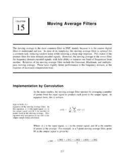
2 There are also systemsthat process segment-by-segment because they operate in real time. Forexample, telephone signals cannot be delayed by more than a few hundredmilliseconds, limiting the amount of data that are available for processing atany one instant. In still other applications, the processing may require that thesignal be segmented. An example is FFT convolution, the main topic of thischapter. The overlap-add method is based on the fundamental technique in DSP: (1)decompose the signal into simple components, (2) process each of thecomponents in some useful way, and (3) recombine the processed componentsinto the final signal . FIGURE 18-1 shows an example of how this is done forthe overlap-add method. FIGURE (a) is the signal to be filtered, while (b) showsthe filter kernel to be used, a windowed-sinc low-pass filter. Jumping to thebottom of the FIGURE , (i) shows the filtered signal , a smoothed version of (a).

3 The key to this method is how the lengths of these signals are affected by theconvolution. When an N sample signal is convolved with an M sampleThe Scientist and Engineer's Guide to digital signal Processing312filter kernel, the output signal is samples long. For instance, the inputN%M&1signal, (a), is 300 samples (running from 0 to 299), the filter kernel, (b), is 101samples (running from 0 to 100), and the output signal , (i), is 400 samples(running from 0 to 399). In other words, when an N sample signal is filtered, it will be expanded by points to the right. (This is assuming that the filter kernel runs fromM&1index 0 to M. If negative indexes are used in the filter kernel, the expansionwill also be to the left). In (a), zeros have been added to the signal betweensample 300 and 399 to illustrate where this expansion will occur. Don't beconfused by the small values at the ends of the output signal , (i).

4 This issimply a result of the windowed-sinc filter kernel having small values near itsends. All 400 samples in (i) are nonzero, even though some of them are toosmall to be seen in the graph. Figures (c), (d) and (e) show the decomposition used in the overlap-addmethod. The signal is broken into segments, with each segment having 100samples from the original signal . In addition, 100 zeros are added to the rightof each segment. In the next step, each segment is individually filtered byconvolving it with the filter kernel. This produces the output segments shownin (f), (g), and (h). Since each input segment is 100 samples long, and thefilter kernel is 101 samples long, each output segment will be 200 sampleslong. The important point to understand is that the 100 zeros were added toeach input segment to allow for the expansion during the convolution.

5 Notice that the expansion results in the output segments overlapping eachother. These overlapping output segments are added to give the outputsignal, (i). For instance, samples 200 to 299 in (i) are found by adding thecorresponding samples in (g) and (h). The overlap-add method producesexactly the same output signal as direct convolution. The disadvantage isa much greater program complexity to keep track of the overlappingsamples. FFT ConvolutionFFT convolution uses the principle that multiplication in the frequencydomain corresponds to convolution in the time domain. The input signal istransformed into the frequency domain using the DFT, multiplied by thefrequency response of the filter, and then transformed back into the timedomain using the Inverse DFT. This basic technique was known since thedays of Fourier; however, no one really cared. This is because the timerequired to calculate the DFT was longer than the time to directly calculatethe convolution.

6 This changed in 1965 with the development of the FastFourier Transform (FFT). By using the FFT algorithm to calculate theDFT, convolution via the frequency domain can be faster than directlyconvolving the time domain signals. The final result is the same; only thenumber of calculations has been changed by a more efficient algorithm. Forthis reason, FFT convolution is also called high-speed convolution. Chapter 18- FFT Convolution313 Sample number0100200300400-4-2024 Sample number0100200300400-4-2024 Sample number0100200300400-4-2024 Sample number0100200300400-4-2024 Sample number0100200300400-4-2024 Sample number0100200300400-4-2024 Sample number0100200300400-4-2024 Sample number0100200300400-4-2024a. Input signalc. Input segment 1f. Output segment 1d. Input segment 2e. Input segment 3h. Output segment 3i. Output signalg. Output segment 2 Filterkernel?addedzerosAmplitudeAmplitud eAmplitudeAmplitudeAmplitudeAmplitudeAmp litudeAmplitudeAmplitudeFIGURE 18-1 The overlap-add method.

7 The goal is to convolve theinput signal , (a), with the filter kernel, (b). This isdone by breaking the input signal into a number ofsegments, such as (c), (d) and (e), each padded withenough zeros to allow for the expansion during theconvolution. Convolving each of the input segmentswith the filter kernel produces the output segments,(f), (g), and (h). The output signal , (i), is then foundby adding the overlapping output segments. The Scientist and Engineer's Guide to digital signal Processing314 FFT convolution uses the overlap-add method shown in Fig. 18-1; only the waythat the input segments are converted into the output segments is 18-2 shows an example of how an input segment is converted into anoutput segment by FFT convolution. To start, the frequency response of thefilter is found by taking the DFT of the filter kernel, using the FFT. Forinstance, (a) shows an example filter kernel, a windowed-sinc band-pass FFT converts this into the real and imaginary parts of the frequencyresponse, shown in (b) & (c).

8 These frequency domain signals may not looklike a band-pass filter because they are in rectangular form. Remember, polarform is usually best for humans to understand the frequency domain, whilerectangular form is normally best for mathematical calculations. These realand imaginary parts are stored in the computer for use when each segment isbeing calculated. FIGURE (d) shows the input segment to being processed. The FFT is used to findits frequency spectrum, shown in (e) & (f). The frequency spectrum of theoutput segment, (h) & (i) is then found by multiplying the filter's frequencyresponse, (b) & (c), by the spectrum of the input segment, (e) & (f). Sincethese spectra consist of real and imaginary parts, they are multiplied accordingto Eq. 9-1 in Chapter 9. The Inverse FFT is then used to find the outputsegment, (g), from its frequency spectrum, (h) & (i).

9 It is important torecognize that this output segment is exactly the same as would be obtained bythe direct convolution of the input segment, (d), and the filter kernel, (a).The FFTs must be long enough that circular convolution does not take place(also described in Chapter 9). This means that the FFT should be the samelength as the output segment, (g). For instance, in the example of Fig. 18-2,the filter kernel contains 129 points and each segment contains 128 points,making output segment 256 points long. This calls for 256 point FFTs to beused. This means that the filter kernel, (a), must be padded with 127 zeros tobring it to a total length of 256 points. Likewise, each of the input segments,(d), must be padded with 128 zeros. As another example, imagine you needto convolve a very long signal with a filter kernel having 600 samples. Onealternative would be to use segments of 425 points, and 1024 point alternative would be to use segments of 1449 points, and 2048 pointFFTs.

10 Table 18-1 shows an example program to carry out FFT convolution. Thisprogram filters a 10 million point signal by convolving it with a 400 point filterkernel. This is done by breaking the input signal into 16000 segments, witheach segment having 625 points. When each of these segments is convolvedwith the filter kernel, an output segment of points is625%400&1'1024produced. Thus, 1024 point FFTs are used. After defining and initializing allthe arrays (lines 130 to 230), the first step is to calculate and store thefrequency response of the filter (lines 250 to 310). Line 260 calls amythical subroutine that loads the filter kernel into XX[0] throughXX[399], and sets XX[400] through XX[1023] to a value of zero. Thesubroutine in line 270 is the FFT, transforming the 1024 samples held inXX[ ] into the 513 samples held in REX[ ] & IMX[ ], the real andChapter 18- FFT Convolution315 Sample Filter kerneld.