Transcription of Finite-Di erence Approximations to the Heat Equation
1 finite -Difference Approximations to the heat Equation Gerald W. Recktenwald . March 6, 2011. Abstract This article provides a practical overview of numerical solutions to the heat Equation using the finite difference method. The forward time, centered space (FTCS), the backward time, centered space (BTCS), and Crank-Nicolson schemes are developed, and applied to a simple problem involving the one-dimensional heat Equation . Complete, working Mat- lab codes for each scheme are presented. The results of running the codes on finer (one-dimensional) meshes, and with smaller time steps is demonstrated. These sample calculations show that the schemes real- ize theoretical predictions of how their truncation errors depend on mesh spacing and time step.
2 The Matlab codes are straightforward and al- low the reader to see the differences in implementation between explicit method (FTCS) and implicit methods (BTCS and Crank-Nicolson). The codes also allow the reader to experiment with the stability limit of the FTCS scheme. 1 The heat Equation The one dimensional heat Equation is 2 . = 2, 0 x L, t 0 (1). t x where = (x, t) is the dependent variable, and is a constant coefficient. Equation (1) is a model of transient heat conduction in a slab of material with thickness L. The domain of the solution is a semi-infinite strip of width L that continues indefinitely in time. The material property is the thermal diffusivity. In a practical computation, the solution is obtained only for a finite time, say tmax.
3 Solution to Equation (1) requires specification of boundary conditions at x = 0 and x = L, and initial conditions at t = 0. Simple boundary and initial conditions are (0, t) = 0 , (L, t) = L (x, 0) = f0 (x). (2). Other boundary conditions, gradient (Neumann) or mixed conditions, can be specified. To keep the presentation as simple as possible, only the conditions in (2) are considered in this article. Associate Professor, Mechanical Engineering Department Portland State University, Port- land, Oregon, 2 finite DIFFERENCE METHOD 2. 2 finite Difference Method The finite difference method is one of several techniques for obtaining numerical solutions to Equation (1). In all numerical solutions the continuous partial differential Equation (PDE) is replaced with a discrete approximation .
4 In this context the word discrete means that the numerical solution is known only at a finite number of points in the physical domain. The number of those points can be selected by the user of the numerical method. In general, increasing the number of points not only increases the resolution ( , detail), but also the accuracy of the numerical solution. The discrete approximation results in a set of algebraic equations that are evaluated (or solved) for the values of the discrete unknowns. Figure 1 is a schematic representation of the numerical solution. The mesh is the set of locations where the discrete solution is computed. These points are called nodes, and if one were to draw lines between adjacent nodes in the domain the resulting image would resemble a net or mesh.
5 Two key parameters of the mesh are x, the local distance between adjacent points in space, and t, the local distance between adjacent time steps. For the simple examples considered in this article x and t are uniform throughout the mesh. In Section the mesh is defined. The core idea of the finite -difference method is to replace continuous deriva- tives with so-called difference formulas that involve only the discrete values associated with positions on the mesh. In Section a handful of difference formulas are developed. Applying the finite -difference method to a differential Equation involves re- placing all derivatives with difference formulas. In the heat Equation there are derivatives with respect to time, and derivatives with respect to space.
6 Us- ing different combinations of mesh points in the difference formulas results in different schemes. In the limit as the mesh spacing ( x and t) go to zero, the numerical solution obtained with any useful1 scheme will approach the true solution to the original differential Equation . However, the rate at which the numerical solution approaches the true solution varies with the scheme. In ad- dition, there are some practically useful schemes that can fail to yield a solution for bad combinations of x and t. Three different schemes for the solution to Equation (1) are developed in Section 3. The numerical solution of the heat Equation is discussed in many textbooks. Ames [1], Morton and Mayers [3], and Cooper [2] provide a more mathematical development of finite difference methods.
7 See Cooper [2] for modern introduc- tion to the theory of partial differential equations along with a brief coverage of numerical methods. Fletcher [4], Golub and Ortega [5], and Hoffman [6] take a more applied approach that also introduces implementation issues. Fletcher provides Fortran code for several methods. The Discrete Mesh The finite difference method obtains an approximate solution for (x, t) at a finite set of x and t. For the codes developed in this article the discrete x are 1 There are plausible schemes that do not exhibit this important property of converging to the true solution. Refer to discussions of consistency in references [1, 2]. 2 finite DIFFERENCE METHOD 3. Continuous finite Discrete Solution difference m i approxi- PDE for Difference method.
8 Mation to (x, t). (x, t) Equation Figure 1: Relationship between continuous and discrete problems. uniformly spaced in the interval 0 x L such that xi = (i 1) x, i = 1, 2, .. N. where N is the total number of spatial nodes, including those on the boundary. Given L and N , the spacing between the xi is computed with L. x = . N 1. Similarly, the discrete t are uniformly spaced in 0 t tmax : tm = (m 1) t, m = 1, 2, .. M. where M is the number of time steps and t is the size of a time step2. tmax t = . M 1. The solution domain is depicted in Figure 2. Table 1 summarizes the notation used to obtain the approximate solution to Equation (1) and to analyze the result. finite Difference Approximations The finite difference method involves using discrete Approximations like i+1 i (3).
9 X x 2 The first mesh lines in space and time are at i = 1 and m = 1 to be consistent with the Matlab requirement that the first row or column index in a vector or matrix is one. Table 1: Notation Symbol Meaning (x, t) Continuous solution (true solution). (xi , tm ) Continuous solution evaluated at the mesh points. m i Approximate numerical solution obtained by solving the finite -difference equations . 2 finite DIFFERENCE METHOD 4. t .. m+1. m m 1. t=0. 1 i 1 i i+1 N. x=0 x=L. Figure 2: Mesh on a semi-infinite strip used for solution to the one-dimensional heat Equation . The solid squares indicate the location of the (known) initial values. The open squares indicate the location of the (known) boundary values. The open circles indicate the position of the interior points where the finite difference approximation is computed.
10 Where the quantities on the right hand side are defined on the finite difference mesh. Approximations to the governing differential Equation are obtained by replacing all continuous derivatives by discrete formulas such as those in Equa- tion (3). The relationship between the continuous (exact) solution and the discrete approximation is shown in Figure 1. Note that computing m i from the finite difference model is a distinct step from translating the continuous problem to the discrete problem. finite difference formulas are first developed with the dependent variable . as a function of only one independent variable, x, = (x). The resulting formulas are then used to approximate derivatives with respect to either space or time.