Transcription of Finite Difference Methods - Massachusetts Institute of ...
1 Chapter 13. Finite Difference Methods In the previous chapter we developed Finite Difference approximations for partial derivatives. In this chapter we will use these Finite Difference approximations to solve partial differential equations (PDEs) arising from conservation law presented in Chapter 11. 48 Self-Assessment Before reading this chapter, you may wish to Conservation Laws 11. Finite Difference Approximations 12. After reading this chapter you should be able implement a Finite Difference method to solve a PDE. compute the order of accuracy of a Finite Difference method develop upwind schemes for hyperbolic equations Relevant self-assessment exercises: 4 - 6. 49 Finite Difference Methods Consider the one-dimensional convection-diffusion equation, U U 2U. +u 2 = 0. (101). t x x Approximating the spatial derivative using the central Difference operators gives the following approximation at node i, dUi + ui 2xUi x2Ui = 0 (102).
2 Dt This is an ordinary differential equation for Ui which is coupled to the nodal values at Ui 1 . Assembling all of the nodal states into a single vector U = (U0 , U1 , .. , Ui 1 , Ui , Ui+1 , .. , UNx 1 , UNx )T , gives a system of coupled ODEs of the form: 67. 68. dU. = AU + b (103). dt where b will contain boundary condition related data (boundary conditions are discussed in Section ). The matrix A has the form: . A0,0 A0,1 .. A0,Nx A1,0 A1,1 .. A1,Nx . A= .. ANx ,0 ANx ,1 .. ANx ,Nx Note that row i of this matrix contains the coefficients of the nodal values for the ODE governing node i. Except for rows requiring boundary condition data, the values of Ai, j are related to the coefficients j of the Finite Difference approximation. Specifically, for our central Difference approximation ui . Ai,i 1 = + 2, 2 x x . Ai,i = 2 2 , x ui . Ai,i+1 = + , 2 x x2. and all other entries in row i are zero.
3 In general, the number of non-zero entries in row i will correspond to the size of the stencil of the Finite Difference approximations used. We refer to Equation 103 as being semi-discrete, since we have discretized the PDE in space but not in time. To make this a fully discrete approximation, we could apply any of the ODE integration Methods that we discussed previously. For example, the simple forward Euler integration method would give, U n+1 U n = AU n + b. (104). t Using central Difference operators for the spatial derivatives and forward Euler integration gives the method widely known as a Forward Time-Central Space (FTCS) approximation. Since this is an explicit method A does not need to be formed explicitly. Instead we may simply update the solution at node i as: 1. Uin+1 = Uin (ui 2xUin x2 Uin ) (105). t Example 1. Finite Difference Method applied to 1-D Convection In this example, we solve the 1-D convection equation, U U.
4 +u = 0, t x using a central Difference spatial approximation with a forward Euler time integration, Uin+1 Uin + uni 2xUin = 0. t Note: this approximation is the Forward Time-Central Space method from Equation 111 with the diffusion terms removed. We will solve a problem that is nearly the same as that in Example 3. Specifically, we use a constant velocity, u = 1 and set the initial condition to be x 2. U0 (x) = ( ) . We consider the domain = [0, 1] with periodic boundary conditions and we will make use of the central Difference approximation developed in Exercise 1. The matlab script which implements this algorithm is: 69. 1 % This Matlab script solves the one-dimensional convection 2 % equation using a Finite Difference algorithm. The 3 % discretization uses central differences in space and forward 4 % Euler in time. 5. 6 clear all;. 7 close all;. 8. 9 % Number of points 10 Nx = 50.
5 11 x = linspace(0,1,Nx+1);. 12 dx = 1/Nx;. 13. 14 % velocity 15 u = 1;. 16. 17 % Set final time 18 tfinal = ;. 19. 20 % Set timestep 21 dt = ;. 22. 23 % Set initial condition 24 Uo = *exp(-(( ) ). 2)';. 25 t = 0;. 26. 27 U = Uo;. 28. 29 % Loop until t > tfinal 30 while (t < tfinal), 31 % Forward Euler step 32 U(2:end) = U(2:end) - dt*u*centraldiff(U(2:end));. 33 U(1) = U(end); % enforce periodicity 34. 35 % Increment time 36 t = t + dt;. 37. 38 % Plot current solution 39 clf 40 plot(x,Uo,'b*');. 41 hold on;. 42 plot(x,U,'*','color',[0 0]);. 43 xlabel('x','fontsize',16); ylabel('U','fontsize',16);. 44 title(sprintf('t = %f\n',t));. 45 axis([0, 1, , ]);. 46 grid on;. 47 drawnow;. 48 end Figure 20 plots the Finite Difference solution at time t = , t = , and t = The exact solution for this problem has U(x,t) = Uo (x) for any integer time (t = 1, 2, ..). When the numerical method is run, the Gaussian disturbance in convected across the domain, however small oscillations are observed at t = which begin to pollute the numerical solution.
6 Eventually, these oscillations grow until the entire solution is contaminated. In Chapter 14 we will show that the FTCS algorithm is unstable for any t for pure convection. Thus, what we are observing is an instability that can be predicted through some analysis. Exercise 1. Download the matlab code from Example 1 and modify the code to use the backward Difference formula x . This method known, as the Forward Time-Backward Space (FTBS) method. Using the same u = 1, t = 1000. 1. and x = 50. 1. does the FTBS method exhibit the same instability as the FTCS method? 70. t = t = t = U U U. o o o U(t) U(t) U(t). 1 1 1. U. U. U. 0 0 0. 0 1 0 1 0 1. x x x (a) t = (b) t = (c) t = Fig. 20 Forward Time-Central Space method for 1-D convection. (a) Yes (b) No (c) Sometimes (d) I don't know Boundary Conditions In this section, we discuss the implementation of Finite Difference Methods at boundaries.
7 This discussion is not meant to be comprehensive, as the issues are many and often subtle. In particular, we only focus on Dirichlet boundary conditions. A Dirichlet boundary condition is one in which the state is specified at the boundary. For example, in a heat transfer problem the temperature may be known at the domain boundaries. Dirichlet boundary conditions can be implemented in a relatively straightforward manner. For example, suppose that we are solving a one-dimensional convection-diffusion problem and we want the value of U at i = 0, to be Uinlet , U0 = Uinlet . To implement this, we fix U0 = Uinlet and apply the Finite Difference discretization only over the interior of the compu- tational domain accounting for the known value of U0 at any place where the interior discretization depends on it. For example, at the first interior node ( i = 1), the central Difference discretization of for the 1-D convection-diffusion equation gives, dU1 U2 U0 U2 2U1 +U0.
8 + u1 = . dt 2 x x2. Accounting for the known value of U0 , this becomes, dU1 U2 Uinlet U2 2U1 +Uinlet + u1 = . (106). dt 2 x x2. In terms of the vector notation, when a Dirichlet boundary condition is applied we usually remove that state from the vector U. So, in the situation where U0 is known, the state vector is defined as, U = (U1 ,U2 , .. , Ui 1 ,Ui ,Ui+1 , .. , UNx 1 ,UNx )T , 71. The b vector then will contain the contributions from the known boundary values. For example, by re-arranging Equation (106), the first row of b contains, Uinlet Uinlet b1 = u2 + . 2 x x2. Since Uinlet does not enter any of the other node's stencils, the remaining rows of b will be zero (unless they are altered by the other boundary). Exercise 2. Download the matlab code from Example 1 and modify the code to use a Dirichlet boundary con- dition on the inflow and the backwards Difference formula x on the outflow.
9 Using the same u = 1, t = 1000. 1. and x = 50 is the FTCS method with Dirichlet boundary condition stable? 1. (a) Yes (b) No (c) Sometimes (d) I don't know Truncation Error for a PDE. In the discussion of ODE integration, we used the ideas of consistency and stability to prove convergence through the Dahlquist Equivalence Theorem. Similar concepts also exist for PDE discretizations, however, we cannot cover these here. We will briefly look at the truncation error for a partial differential equation. We have already discussed the local truncation error for Finite Difference approximation of derivatives in Section Similar to the ODE case, the truncation error is defined as the remainder after an exact solution to the governing equation is substituted into the Finite Difference approximation. For example, suppose we are using the FTCS algorithm in Equation 111 to approximate the one-dimensional convection-diffusion equation.
10 Then the local truncation error for the PDE approximation is defined as, Uin+1 Uin + uni 2xUin x2 Uin , (107). t where U(x,t) is an exact solution to Equation (94). Note that the truncation error defined here for PDE's is not quite a direct analogy with the standard definition of local truncation error used in ODE integration, specifically in Equation (16). In particular, in the ODE case, the truncation error is defined as the Difference between the numerical solution and the exact solution after one step of the method (starting from exact values). However, in the PDE case, we have defined the truncation error as the remainder after an exact solution is substituted into the numerical method when the numerical method is written in a form that approximates the governing PDE. Except for this Difference in the definition, the calculation of the local truncation follows the same procedure as in the ODE case in which Taylor series substitutions are used to expand the error in powers of t.