Transcription of FINITE ELEMENT METHODS FOR MAXWELL EQUATIONS
1 FINITE ELEMENT METHODS FOR MAXWELL EQUATIONSLONG CHENABSTRACT. We give a brief introduction to FINITE ELEMENT METHODS for solving that the time-harmonic MAXWELL equation for electric fieldEis ( 1 E) 2 E= J ( E) = .The time-harmonic MAXWELL equation for magnetic fieldHis ( 1 H) 2 H= J ( H) = are obtained by Fourier transform in time for the original MAXWELL EQUATIONS . Here is a positive constant called the frequency. For derivation and physical meaning, we refertoBrief Introduction to MAXWELL s EQUATIONS . In this note, we shall consider FINITE elementmethods for solving time-harmonic MAXWELL INTRODUCTIONLet be a bounded Lipschitz domain inR3. We introduce the Sobolev spacesH(curl ; ) ={v L2( ),curlv L2( )},H(div; ) ={v L2( ),divv L2( )}The intensity fields(E,H)belong toH(curl ; )while the flux field(D,B)inH(div; ).
2 We use the unified notationH(d; )withd = grad,curl,ordiv. Note thatH(grad ; )is the familiarH1( )space. One can verify thatH(d; )is a Hilbert space with respectto the inner product(u,v) + ( du,dv).The norm forH(d; )is the graph norm u d, :=( u 2+ du 2)1 recall the integration by parts for vector functions below. Formally the boundaryterm is obtained by replacing the Hamilton operator by the unit outwards normal vectorDate: Created: Spring 2014. Last update: July 18, CHENn. For example, u dx= u dx+ nu dS, u dx= u dx+ n u dS, u dx= u dx+ n u weak formulation is obtained by multiplying the original equation by a smooth testequation and applying the integration by parts. The boundary condition will be discussedlater. For time-harmonic MAXWELL EQUATIONS , the weak formulation forEis(1)( 1 E, ) 2( E, ) = ( J, ) D( ).
3 And the equation forHis(2)( 1 H, ) 2( H, ) = ( J, ) D( ).In (2) the source Jis understood in the distribution sense and , as the adjointof itself, is moved to the test function. The coefficient and the current Jare in generalcomplex functions and so areE, divergence constraint is build into the weak formulation when 6= 0. For example,the conditiondiv( H) = 0in the distribution sense can be obtained by applyingdivoperator to the equation ( 1 H) 2 H= J. When = 0, we need toimpose the constraint explicitly; see (4).To simplify the discussion, we consider the following model problems: Symmetric and positive definite problem:(3) ( u) + u=fin ,u n= 0on Saddle point system:(4) ( u) =fin , ( u) = 0in ,u n= 0on .where and are uniformly bounded and positive and real coefficients.
4 The right handsidefis divergence free, 0in the distribution INTERFACE ANDBOUNDARYCONDITIONSFor a vectoru R3and a unit norm vectorn, we can decomposeuinto the normalcomponent and the tangential component asu= (u n)n+n (u n) =un+u .The vectoru nis also on the tangent plane and orthogonal to the tangential componentu which is a clockwise90 rotation ofu on the tangent plane. Consequently{u n,u ,n}forms an orthogonal basis ofR3; see Fig. interface condition can be derived from the continuity requirement for piecewisesmooth functions to be inH(d; ). Let =K1 K2 Swith interfaceS= K1 H(d;Ki). Defineu L2( )asu={u1x K1,u2x ELEMENT METHODS FOR MAXWELL Negative Index Media7and may be thought of as thesourcesof the fields in Eq. ( ). In Sec. , we examinethis interpretation further and show how it leads to the Ewald-Oseen extinction theoremand to a microscopic explanation of the origin of the refractive Negative Index MediaMaxwell s EQUATIONS do not preclude the possibility that one or both of the quantities!}
5 , be negative. For example, plasmas below their plasma frequency, and metals up tooptical frequencies, have!<0 and >0, with interesting applications such as surfaceplasmons (see Sec. ).Isotropic media with <0 and!>0 are more difficult to come by [153], althoughexamples of such media have been fabricated [381].Negative-index media, also known as left-handed media, have!, that are simulta-neously negative,!<0 and <0. Veselago [376] was the first to study their unusualelectromagnetic properties, such as having a negative index of refraction and the rever-sal of Snel s novel properties of such media and their potential applications have generateda lot of research interest [376 457]. Examples of such media, termed metamaterials ,have been constructed using periodic arrays of wires and split-ring resonators, [382]and by transmission line elements [415 417,437,450], and have been shown to exhibitthe properties predicted by !
6 Rel<0 and rel<0, the refractive index,n2=!rel rel, must be defined bythe negative square rootn= !rel rel. Because thenn<0 and rel<0 will implythat the characteristic impedance of the medium = 0 rel/nwill be positive, whichas we will see later implies that the energy flux of a wave is in the same direction as thedirection of propagation. We discuss such media in Sections , , and Boundary ConditionsThe boundary conditions for the electromagnetic fields across material boundaries aregiven below:E1t E2t=0H1t H2t=Js nD1n D2n= sB1n B2n=0( )where nis a unit vector normal to the boundary pointing from medium-2 into quantities s,Jsare any externalsurface chargeandsurface currentdensities onthe boundary surface and are measured in units of [coulomb/m2] and [ampere/m].In words, thetangentialcomponents of theE-field are continuous across the inter-face; the difference of thetangentialcomponents of theH-field are equal to the surface81.
7 MAXWELL s Equationscurrent density; the difference of thenormalcomponents of the flux densityDare equalto the surface charge density; and thenormalcomponents of the magnetic flux densityBare condition may also be written a form that brings out the depen-dence on the polarization surface charges:(!0E1n+P1n) (!0E2n+P2n)= s !0(E1n E2n)= s P1n+P2n= s,totThe total surface charge density will be s,tot= s+ 1s,pol+ 2s,pol, where the surfacecharge density of polarization charges accumulating at the surface of a dielectric is seento be ( nis the outward normal from the dielectric): s,pol=Pn= n P( )The relative directions of the field vectors are shown in Fig. Each vector maybe decomposed as the sum of a part tangential to the surface and a part perpendicularto it, that is,E=Et+En. Using the vector identity,E= n (E n)+ n( n E)=Et+En( )we identify these two parts as:Et= n (E n),En= n( n E)= nEnFig.
8 Directions at these results, we can write the first two boundary conditions in the followingvectorial forms, where the second form is obtained by taking the cross product of thefirst with nand noting thatJsis purely tangential: n (E1 n) n (E2 n)=0 n (H1 n) n (H2 n)=Js nor, n (E1 E2)=0 n (H1 H2)=Js( )The boundary conditions ( ) can be derived from the integrated form of MAXWELL sequations if we make some additional regularity assumptions about the fields at Field directions at boundary. Extract fromElectromagneticWaves and Antennasby Orfanidis [9].We can always define derivativeduin the distribution sense. To be a weak derivative, weneed to verify it coincides with the piecewise derivative, ,du={du1x K1,du2x do so, let D( ), by the definition of the derivative of a distribution du, := u,d = (u1,d ) + (u2,d )= ( du1, ) + ( du2, ) + S(u1 u2), S,whered is the adjoint ofdinL2-inner product and Sis an appropriate restriction offunctions on the interface depending on the differential operators.}
9 The negative sign infront ofu2is from the fact the outwards normal direction ofK2is opposite to that H(d; )if and only if u1|S=u2|Sford = grad,n u1|S=n u2|Sford = curl,n u1|S=n u2|Sford = strictly speaking, the restriction operator( )|Sshould be replaced by appropriate traceoperators which will be discussed in the next for a function inH(curl ; ), its tangential component should be continuous acrossthe interface and for a function inH(div; ), its normal component should be will be the key of constructing FINITE ELEMENT spaces for these Sobolev the interfaceScontains surface charge Sand surface currentJS, the interfacecondition forHandDis changed to(H1 H2) n=JS,(D1 D2) n= interface condition forHcan be build into the right hand side of the weak formulation(2) using a surface integral boundary condition can be thought of as an interface condition when one side of theinterface is the free space.
10 The following are popular boundary conditions for MAXWELL -type EQUATIONS . If one side is a perfect conductor, then = . By Ohm s law, to have a finitecurrent, the electric fieldEshould be zero. So we obtain the boundary conditionE n= 0for a perfect conductor. Impedance boundary condition 1 1more on thisn H Et= CHEN3. TRACESThe trace of functions inH(d; )is not simply the restriction of the function valuessince the differential operatordivorcurlcontrols only partial component of the vectorfunction. The best way to look at the trace is, again, through integration by that :H1( ) H1/2( )is the trace operator forH1functions. It iscontinuous and surjective. Whenuis also continuous on , u=u| . (div; ) functionsv C1( ), C1( )and is a domain withsmooth boundary, we have the following integration by parts(5) divv dx= v grad dx+ n v we relax the smoothness of functions and the domain such that (5) still holds.