Transcription of First Order Partial Differential Equations
1 1 First Order Partial Differential Equations The profound study of nature is the most fertile source of mathematical discover-ies. - Joseph Fourier (1768-1830) begin our study of Partial Differential equationswithfirstorder Partial Differential doing so, we need to define a (see the appendix on Differential Equations ) that ann-th orderordinary Differential equation is an equation for an unknown functiony(x)n-th Order ordinary Differential equationthat expresses a relationship between the unknown function and its firstnderivatives. One could write this generally asF(y(n)(x),y(n 1)(x).)
2 ,y (x),y(x),x) =0.( )Herey(n)(x)represents thenth derivative ofy(x). Furthermore, and initialvalue problem consists of the Differential equation plus the values of theInitial value 1 derivatives at a particular value of the independent variable, sayx0:y(n 1)(x0) =yn 1,y(n 2)(x0) =yn 2,.. ,y(x0) =y0.( )If conditions are instead provided at more than one value of the indepen-dent variable, then we have a boundary value problem..If the unknown function is a function of several variables, then the deriva-tives are Partial derivatives and the resulting equation is a Partial differen-tial equation.
3 Thus, ifu=u(x,y, ..), a general Partial Differential equationmight take the formF(x,y, .. ,u, u x, u y, .. , 2u x2, ..)=0.( )Since the notation can get cumbersome, there are different ways to writethe Partial derivatives. First Order derivatives could be written as u x,ux, xu, Partial Differential equationsSecond Order Partial derivatives could be written in the forms 2u x2,uxx, xxu,D2xu. 2u x y= 2u y x,uxy, xyu, , we are assuming thatu(x,y, ..)has continuous Partial , according to Clairaut s Theorem (Alexis Claude Clairaut,1713-1765) ,mixed Partial derivatives are the of some of the Partial Differential equation treated in this bookare shown in However, being that the highest Order derivatives inthese equation are of second Order , these are second Order Partial differentialequations.
4 In this chapter we will focus on First Order Partial differentialequations. Examples are given byut+ux= +uux= +uux= 2uy+u= function of two variables, which the above are examples, a generalfirst Order Partial Differential equation foru=u(x,y)is given asF(x,y,u,ux,uy) =0,(x,y) D R2.( )This equation is too general. So, restrictions can be placed on the form,leading to a classification of First Order Equations . A linear First Order partialdifferential equation is of the formLinear First Order Partial (x,y)ux+b(x,y)uy+c(x,y)u=f(x,y).( )Note that all of the coefficients are independent ofuand its derivatives andeach term in linear inu,ux, can relax the conditions on the coefficients a bit.
5 Namely, we could as-sume that the equation is linear only inuxanduy. This gives the quasilinearfirst Order Partial Differential equation in the formQuasilinear First Order Partial (x,y,u)ux+b(x,y,u)uy=f(x,y,u).( )Note that theu-term was absorbed byf(x,y,u).In between these two forms we have the semilinear First Order partialdifferential equation in the formSemilinear First Order Partial (x,y)ux+b(x,y)uy=f(x,y,u).( )Here the left side of the equation is linear inu,uxanduy. However, the righthand side can be nonlinear the most part, we will introduce the Method of Characteristics forsolving quasilinear Equations .
6 But, let us First consider the simpler case oflinear First Order constant coefficient Partial Differential Order Partial Differential Equations Constant Coefficient EquationsLet s consider the linear First Order constant coefficientpar-tial Differential equationaux+buy+cu=f(x,y),( )fora,b, andcconstants witha2+b2>0. We will consider how such equa-tions might be solved. We do this by considering two cases,b=0 andb6= the First case,b=0, we have the equationaux+cu= can view this as a First Order linear (ordinary) Differential equation withya parameter. Recall that the solution of such Equations can be obtainedusing an integrating factor.
7 [See the discussion after Equation ( ).] Firstrewrite the equation asux+cau= the integrating factor (x) =exp( xcad ) =ecax,the Differential equation can be written as( u)x=fa .Integrating this equation and solving foru(x,y), we have (x)u(x,y) =1a f( ,y) ( )d +g(y)ecaxu(x,y) =1a f( ,y)eca d +g(y)u(x,y) =1a f( ,y)eca( x)d +g(y)e cax.( )Hereg(y)is an arbitrary function the second case,b6=0, we have to solve the equationaux+buy+cu= would help if we could find a transformation which would eliminate oneof the derivative terms reducing this problem to the previous case. That iswhat we will First note thataux+buy= (ai+bj) (uxi+uyj)= (ai+bj) u.
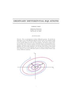
8 ( )4 Partial Differential equationsRecall from multivariable calculus that the last term is nothing but a direc-tional derivative ofu(x,y)in the directionai+bj. [Actually, it is propor-tional to the directional derivative ifai+bjis not a unit vector.]Therefore, we seek to write the Partial Differential equation as involving aderivative in the directionai+bjbut not in a directional orthogonal to depict a new set of coordinates in which thewdirection isorthogonal toai+ ayai+ : Coordinate systems for trans-formingaux+buy+cu=fintobvz+cv=fusi ng the transformationw=bx ayandz= consider the transformationw=bx ay,z=y.
9 ( )We First note that this transformation is invertible,x=1b(w+az),y=z.( )Next we consider how the derivative terms transform. Letu(x,y) =v(w,z). Then, we haveaux+buy=a xv(w,z) +b yv(w,z),=a[ v w w x+ v z z x]+b[ v w w y+ v z z y]=a[bvw+0 vz] +b[ avw+vz]=bvz.( )Therefore, the Partial Differential equation becomesbvz+cv=f(1b(w+az),z).This is now in the same form as in the First case and can be solved using anintegrating the general solution of the equation3ux 2uy+u= , we transform the equation into new ay= 2x 3y,and z= ,ux 2uy=3[ 2vw+0 vz] 2[ 3vw+vz]= 2vz.( )The new Partial Differential equation for v(w,z)is 2 v z+v=x= 12(w+3z).
10 First Order Partial Differential Equations 5 Rewriting this equation, v z 12v=14(w+3z),we identify the integrating factor (z) =exp[ z12d ]=e this integrating factor, we can solve the Differential equation for v(w,z). z(e z/2v)=14(w+3z)e z/2,e z/2v(w,z) =14 z(w+3 )e /2d = 12(w+6+3z)e z/2+c(w)v(w,z) = 12(w+6+3z) +c(w)ez/2u(x,y) =x 3+c( 2x 3y)ey/2.( ) Equations : The Method of InterpretationWe consider the quasilinear Partial Differential equationintwo independent variables,a(x,y,u)ux+b(x,y,u)uy c(x,y,u) =0.( )Letu=u(x,y)be a solution of this equation. Then,f(x,y,u) =u(x,y) u=0describes the solution surface, or integral surface,Integral recall from multivariable, or vector, calculus that the normal to theintegral surface is given by the gradient function, f= (ux,uy, 1).