Transcription of FLOW IN PIPES - kau
1 11/4/04 7:13 PM Page 321. CHAPTER. FLOW IN PIPES 8. F. luid flow in circular and noncircular PIPES is commonly encountered in practice. The hot and cold water that we use in our homes is pumped OBJECTIVES. through PIPES . Water in a city is distributed by extensive piping net- When you finish reading this chapter, you works. Oil and natural gas are transported hundreds of miles by large should be able to pipelines. Blood is carried throughout our bodies by arteries and veins. The Have a deeper understanding of cooling water in an engine is transported by hoses to the PIPES in the radia- laminar and turbulent flow in tor where it is cooled as it flows . Thermal energy in a hydronic space heat- PIPES and the analysis of fully developed flow ing system is transferred to the circulating water in the boiler, and then it is Calculate the major and minor transported to the desired locations through PIPES .
2 Losses associated with pipe Fluid flow is classified as external and internal, depending on whether the flow in piping networks and fluid is forced to flow over a surface or in a conduit. Internal and external determine the pumping power flows exhibit very different characteristics. In this chapter we consider inter- requirements nal flow where the conduit is completely filled with the fluid, and flow is Understand the different velocity driven primarily by a pressure difference. This should not be confused with and flow rate measurement open-channel flow where the conduit is partially filled by the fluid and thus techniques and learn their the flow is partially bounded by solid surfaces, as in an irrigation ditch, and advantages and disadvantages flow is driven by gravity alone. We start this chapter with a general physical description of internal flow and the velocity boundary layer.
3 We continue with a discussion of the dimensionless Reynolds number and its physical significance. We then dis- cuss the characteristics of flow inside PIPES and introduce the pressure drop correlations associated with it for both laminar and turbulent flows . Then we present the minor losses and determine the pressure drop and pumping power requirements for real-world piping systems. Finally, we present an overview of flow measurement devices. 321. 11/4/04 7:13 PM Page 322. 322. FLUID MECHANICS. 8 1 . INTRODUCTION. Liquid or gas flow through PIPES or ducts is commonly used in heating and cooling applications and fluid distribution networks. The fluid in such appli- cations is usually forced to flow by a fan or pump through a flow section. We pay particular attention to friction, which is directly related to the pres- sure drop and head loss during flow through PIPES and ducts.
4 The pressure drop is then used to determine the pumping power requirement. A typical piping system involves PIPES of different diameters connected to each other by various fittings or elbows to route the fluid, valves to control the flow rate, and pumps to pressurize the fluid. The terms pipe , duct, and conduit are usually used interchangeably for flow sections. In general, flow sections of circular cross section are referred to as PIPES (especially when the fluid is a liquid), and flow sections of non- Circular pipe circular cross section as ducts (especially when the fluid is a gas). Small- diameter PIPES are usually referred to as tubes. Given this uncertainty, we will use more descriptive phrases (such as a circular pipe or a rectangular duct) whenever necessary to avoid any misunderstandings. Water You have probably noticed that most fluids, especially liquids, are trans- 50 atm ported in circular PIPES .
5 This is because PIPES with a circular cross section can withstand large pressure differences between the inside and the outside without undergoing significant distortion. Noncircular PIPES are usually Rectangular used in applications such as the heating and cooling systems of buildings duct where the pressure difference is relatively small, the manufacturing and installation costs are lower, and the available space is limited for ductwork (Fig. 8 1). Although the theory of fluid flow is reasonably well understood, theoreti- Air cal solutions are obtained only for a few simple cases such as fully devel- atm oped laminar flow in a circular pipe . Therefore, we must rely on experimen- FIGURE 8 1 tal results and empirical relations for most fluid flow problems rather than Circular PIPES can withstand large closed-form analytical solutions.
6 Noting that the experimental results are pressure differences between the obtained under carefully controlled laboratory conditions and that no two inside and the outside without systems are exactly alike, we must not be so naive as to view the results undergoing any significant distortion, obtained as exact. An error of 10 percent (or more) in friction factors cal- but noncircular PIPES cannot. culated using the relations in this chapter is the norm rather than the exception.. The fluid velocity in a pipe changes from zero at the surface because of Vavg the no-slip condition to a maximum at the pipe center. In fluid flow, it is convenient to work with an average velocity Vavg, which remains constant in incompressible flow when the cross-sectional area of the pipe is constant (Fig. 8 2). The average velocity in heating and cooling applications may change somewhat because of changes in density with temperature.
7 But, in practice, we evaluate the fluid properties at some average temperature and treat them as constants. The convenience of working with constant proper- ties usually more than justifies the slight loss in accuracy. FIGURE 8 2 Also, the friction between the fluid particles in a pipe does cause a slight Average velocity Vavg is defined as the rise in fluid temperature as a result of the mechanical energy being con- average speed through a cross section. verted to sensible thermal energy. But this temperature rise due to frictional For fully developed laminar pipe flow, heating is usually too small to warrant any consideration in calculations and Vavg is half of maximum velocity. thus is disregarded. For example, in the absence of any heat transfer, no 11/4/04 7:13 PM Page 323. 323. CHAPTER 8. noticeable difference can be detected between the inlet and outlet tempera- tures of water flowing in a pipe .
8 The primary consequence of friction in Turbulent fluid flow is pressure drop, and thus any significant temperature change in flow the fluid is due to heat transfer. The value of the average velocity Vavg at some streamwise cross-section is determined from the requirement that the conservation of mass principle be satisfied (Fig. 8 2). That is, Laminar flow #. m rVavg A c ru(r) dA. Ac c (8 1).. where m is the mass flow rate, r is the density, Ac is the cross-sectional area, and u(r) is the velocity profile. Then the average velocity for incompressible flow in a circular pipe of radius R can be expressed as R. ru(r) dA c ru(r)2pr dr R.. Ac 0 2. Vavg u(r)r dr (8 2). rA c rpR2 R2 0. Therefore, when we know the flow rate or the velocity profile, the average velocity can be determined easily. 8 2 . LAMINAR AND TURBULENT flows FIGURE 8 3. If you have been around smokers, you probably noticed that the cigarette Laminar and turbulent flow regimes smoke rises in a smooth plume for the first few centimeters and then starts of candle smoke.
9 Fluctuating randomly in all directions as it continues its rise. Other plumes behave similarly (Fig. 8 3). Likewise, a careful inspection of flow in a pipe reveals that the fluid flow is streamlined at low velocities but turns chaotic Dye trace as the velocity is increased above a critical value, as shown in Fig. 8 4. The flow regime in the first case is said to be laminar, characterized by smooth streamlines and highly ordered motion, and turbulent in the second case, Vavg where it is characterized by velocity fluctuations and highly disordered motion. The transition from laminar to turbulent flow does not occur sud- denly; rather, it occurs over some region in which the flow fluctuates between laminar and turbulent flows before it becomes fully turbulent. Most Dye injection flows encountered in practice are turbulent. Laminar flow is encountered (a) Laminar flow when highly viscous fluids such as oils flow in small PIPES or narrow passages.
10 We can verify the existence of these laminar, transitional, and turbulent Dye trace flow regimes by injecting some dye streaks into the flow in a glass pipe , as the British engineer Osborne Reynolds (1842 1912) did over a century ago. Vavg We observe that the dye streak forms a straight and smooth line at low velocities when the flow is laminar (we may see some blurring because of molecular diffusion), has bursts of fluctuations in the transitional regime, and zigzags rapidly and randomly when the flow becomes fully turbulent. These Dye injection zigzags and the dispersion of the dye are indicative of the fluctuations in the (b) Turbulent flow main flow and the rapid mixing of fluid particles from adjacent layers. The intense mixing of the fluid in turbulent flow as a result of rapid fluctu- FIGURE 8 4. ations enhances momentum transfer between fluid particles, which increases The behavior of colored fluid injected the friction force on the surface and thus the required pumping power.