Transcription of FOURIER ANALYSIS: LECTURE 6
1 FOURIER analysis : LECTURE Convergence of FOURIER seriesFourier series (real or complex) are very good ways of approximating functions in a finite range, bywhich we mean that we can get a good approximation to the function by using only the first fewmodes ( truncating the sum overnafter some low valuen=N).This is how music compression works in MP3 players, or how digital images are compressed inJPEG form: we can get a good approximation to the true waveform by using only a limited numberof modes, and so all the modes below a certain amplitude are simply saw a related example of this in our approximation to using Eqn. ( ) and Table examinable:Mathematically, this translates as the FOURIER components converging to zero ,bn!0asn!1,providedf(x) is bounded ( has no divergences). But how quickly do the high ordercoe cients vanish? There are two common function and its firstp 1derivatives(f(x),f0(x).)
2 F(p 1)(x)) are continuous, but thepthderivativef(p)(x)hasdiscontinuitie s:an,bn 1/np+1for largen.( )An example of this was our expansion off(x)=x2. When we periodically extend the function,there is a discontinuity in the gradient (p=1derivative)attheboundariesx= seenan 1/n2as expected (withbn=0). (x) is periodic and piecewise continuous ( it has jump discontinuities, but only a finitenumber within one period):)an,bn 1/nfor largen.( )An example of this is the expansion of the odd functionf(x)=x,whichjumpsattheboundary. The FOURIER components turn out to bebn 1/n(withan=0).End of non-examinable How close does it get? Convergence of FOURIER expansionsWe have seen that the FOURIER components generally get smaller as the mode we truncate the FOURIER series afterNterms, we can define an errorDNthat measures how muchthe truncated FOURIER series di ers from the original function: iffN(x)=a02+NXn=1hancos n xL +bnsin n xL i.
3 ( )we define the error asDN=ZL Ldx|f(x) fN(x)|2 0.( )19 Figure : The Gibbs phenomenon for truncated FOURIER approximations to the signum functionEqn. Note the di erentx-range in the lower two is, we square the di erence between the original function and the truncated FOURIER series ateach pointx, ,thisis what is known as things you should know, but which we will not prove: iffis reasonably well-behaved (no non-integrable singularities, and only a finite number of discontinuities), the FOURIER series is optimal inthe least-squares sense if we ask what FOURIER coe cients will minimiseDNfor some givenN, they are exactly the coe cients that we obtain by solving the full FOURIER , asN!1,DN!0. This sounds like we are guaranteed that the FOURIER series willrepresent the function exactly in the limit of infinitely many terms. But looking at the equation forDN,itcanbeseenthatthisisnotso:it salwayspossibletohave(say)fN=2fover some range x,andthebestwecansayisthat xmust tend to zero :As an example of how FOURIER series converge (or not), consider the signum functionwhich picks out the sign of a variable:f(x)=signumx=( 1ifx<0,+1 ifx 0,( )20 NDN10 2: ErrorDNon theN-term truncated FOURIER series approximation to the signum functionEqn.)
4 We will expand in the range 1 x 1( ). Thefunctionisodd,soan=0and we findbn=2Z10dxsin(n x)=2n [1 ( 1)n].( )f(x)hasdiscontinuitiesatx=0andx= L= 1 (due to the periodic extension), so fromSec. we expectedan 1 Table 2 we show the errorDNfor the signum function for increasing values ofDN. As expectedthe error decreases asNgets larger, but relatively slowly. We ll see why this is in the next Ringing artefacts and the Gibbs phenomenonWe saw above that we can define an error associated with the use of a truncated FOURIER series ofNterms to describe a function. Note thatDNmeasures the total error by integrating the deviationat each value ofxover the full range. It does not tell us whether the deviations betweenfN(x)andf(x)werelargeandconcentra tedatcertainvaluesofx,orsmallerandmoreev enlydistributedover all the full interesting case is when we try to describe a function with a finite discontinuity ( a jump)using a truncated FOURIER series , such as our discussion of the signum function Fig.
5 We plot the original functionf(x) that the truncated sum works well, except near the discontinuity. Here the function overshootsthe true value and then has a damped oscillation . As we increaseNthe oscillating region getssmaller, but the overshoot remains roughly the same size (about 18%).This overshoot is known as theGibbs ,wecanseethatittendstobe associated with extended oscillations either side of the step, known as ringing artefacts . Suchartefacts will tend to exist whenever we try to describe sharp transitions with FOURIER methods, andare one of the reasons that MP3s can sound bad when the compression uses too few modes. We canreduce the e ect by using a smoother method of FOURIER series summation, but this is well beyondthis course. For the interested, there are some more details Parseval s theoremThere is a useful relationship between the mean square value of the functionf(x)andtheFouriercoe cients.
6 Parseval s formula is12 LZL L|f(x)|2dx=|a0/2|2+121Xn=1 |an|2+|bn|2 ,( )21or, for complex FOURIER series ,12 LZL L|f(x)|2dx=1Xn= 1|cn|2.( )The simplicity of the expression in the complex case is an example of the advantage of doing thingsthis quantity|cn|2is known as thepower spectrum. This is by analogy with electrical circuits, wherepower like the average power, and|cn|2shows how this is contributedby the di erent FOURIER Parseval is easier in the complex case, so we will stick to this. The equivalent for thesin+cos series is included for interest, but is not examinable. First, note that|f(x)|2=f(x)f (x)and expandfandf as complex FOURIER series :|f(x)|2=f(x)f (x)=1Xn= 1cn n(x)Xmc m m(x)( )(recall that n(x)=eiknx). Then we integrate over L x L,notingtheorthogonalityof nand m:ZL L|f(x)|2dx=1Xm,n= 1cnc mZL L n(x) m(x)dx( )=1Xm,n= 1cnc m(2L mn)=2L1Xn= 1cnc n=2L1Xn= 1|cn|2where we have used the orthogonality relationRL L n(x) m(x)dx=2 Lifm=n, Summing series via ParsevalConsider once again the case off= stheoremis(1/2L)RL Lx4dx=(1/5) complex coe cients were derived earlier, so the sum on the rhs of Parseval s theorem is1Xn= 1|cn|2=|c0|2+Xn6=0|cn|2= L23 2+21Xn=1 2L2( 1)nn2 2 2=L49+1Xn=18L4n4 4.
7 ( )Equating the two sides of the theorem, we therefore get1Xn=11m4=( 4/8)(1/5 1/9) = 4/90.( )This is a series that converges faster than the ones we obtained directly from the series at specialvalues ofx22 FOURIER analysis : LECTURE 73 FOURIER TransformsLearning outcomesIn this section you will learn about FOURIER transforms: their definition and relation to Fourierseries; examples for simple functions; physical examples of their use including the di raction andthe solution of di erential will learn about the Dirac delta function and the convolution of FOURIER transforms as a limit of FOURIER seriesWe have seen that a FOURIER series uses a complete set of modes to describe functions on a finiteinterval the shape of a string of length`.Inthenotationwehaveusedsofar,`= , it is easier to work with`,whichwedobelow;butmosttextbookstra ditionallycoverFourierseries over the range 2L, transforms (FTs) are an extension of FOURIER series that can be used to describe nonperiodicfunctions on an infinite interval.
8 The key idea is to see that a non-periodic function can be viewedas a periodic one, but taking the limit of`! a number of di erent periodic extensions of a given function. This is illustrated in for the case of a square pulse that is only non-zero between a<x<+a. When`becomeslarge compared toa,theperiodicreplicasofthepulsearewide lyseparated,andinthelimitof`!1we have a single isolated pulse. a aFigure : Di erent periodic extensions of a square pulse that is only non-zero between a<x<+a. As the period of the extension,`,increases,thecopiesofthepuls ebecomemorewidelyseparated. In the limit of`!1,wehaveasingleisolatedpulseandtheFo urierseriesgoesoverto the FOURIER series only include modes with wavenumberskn=2n `with adjacent modes separated by k=2 `. What happens to our FOURIER series if we let`!1?Consideragainthecomplexseriesforf (x):f(x)=1Xn= 1 Cneiknx,( )where the coe cients are given byCn=1`Z`/2 `/2dx f(x)e iknx.
9 ( )and the allowed wavenumbers arekn=2n /`.Theseparationofadjacentwavenumbers( !n+1)is k=2 /`;soas`!1, limit, we are then interested in the variation ofCas a function of the continuous factor 1/`outside the integral looks problematic for talking the limit`!1, but this can beevaded by defining a new quantity: f(k) ` C(k)=Z1 1dx f(x)e ikx.( )The function f(k)(o ciallycalled ftilde ,butmorecommonly ftwiddle ;fkis another commonnotation) is theFourier transformof the non-periodic complete the story, we need theinverse FOURIER transform:thisgivesusbackthefunctionf(x) if we know f. Here, we just need to rewrite the FOURIER series , remembering the mode spacing k=2 /`:f(x)=XknC(k)eikx=Xkn(`/2 )C(k)eikx k=12 Xkn f(k)eikx k.( )In this limit, the final form of the sum becomes an integral overk:Xg(k) k!Zg(k)dkas k!0;( )this is how integration gets defined in the first place.
10 We can now write an equation forf(x)inwhich`does not appear:f(x)=12 Z1 1dk f(k)eikx.( )Note the infinite range of integration ink:thiswasalreadypresentintheFourierser ies,wherethemode numbernhad no TIP:You may be asked to explain how the FT is the limit of a FOURIER series (for perhaps6or7marks),somakesureyoucanreprod ucethestu density of statesIn the above, our sum was over individual FOURIER modes. But ifC(k)isacontinuousfunctionofk, we may as well add modes in bunches over some bin ink,ofsize k:f(x)=XkbinC(k)eikxNbin,( )24whereNbinis the number of modes in the bin. What is this? It is just kdivided by the modespacing, 2 /`,sowehavef(x)=`2 XkbinC(k)eikx k( )The term`/2 is thedensity of states:ittellsushowmanymodesexistinunitr angeofk. This isawidelyusedconceptinmanyareasofphysics , ,wecantake the limit of k! (x)anditsFouriertransform f(k)arethereforerelatedby:f(x)=12 Z1 1dk f(k)eikx;( ) f(k)=Z1 1dx f(x)e ikx.