Transcription of Frequency Response - MIT Mathematics
1 Frequency Response 1. Introduction We will examine the Response of a second order linear constant coefficient system to a sinusoidal input. We will pay special attention to the way the output changes as the Frequency of the input changes. This is what we mean by the Frequency Response of the system. In particular, we will look at the amplitude Response and the phase Response ; that is, the amplitude and phase lag of the system's output considered as functions of the input Frequency . In the Exponential Input Theorem was used to find a particular solution in the case of exponential or sinusoidal input. Here we will work out in detail the formulas for a second order system.
2 We will then interpret these formulas as the Frequency Response of a mechanical system. In particular, we will look at damped-spring-mass systems. We will study carefully two cases: first, when the mass is driven by pushing on the spring and second, when the mass is driven by pushing on the dashpot. Both these systems have the same form p ( D ) x = q ( t ), but their amplitude responses are very different. This is because, as we will see, it can make physical sense to designate something other than q(t) as the input. For example, in the system mx 0 + bx 0 + kx = by0. we will consider y to be the input. (Of course, y is related to the expression on the right- hand-side of the equation, but it is not exactly the same.)
3 2. Sinusoidally Driven Systems: Second Order Constant Coefficient DE's We start with the second order linear constant coefficient (CC) DE, which as we've seen can be interpreted as modeling a damped forced harmonic oscillator. If we further specify the oscillator to be a mechanical system with mass m, damping coefficient b, spring constant k, and with a sinusoidal driving force B cos t (with B constant), then the DE is mx 00 + bx 0 + kx = B cos t. (1). For many applications it is of interest to be able to predict the periodic Response of the system to various values of . From this point of view we can picture having a knob you can turn to set the input Frequency , and a screen where we can see how the shape of the system Response changes as we turn the -knob.
4 The Exponential Input Theorem ( (4), and see example 2) tells us how to find a particular solution to (1): Characteristic polynomial: p(r ) = mr2 + br + k. Complex replacement: m x 00 + b x 0 + k x = Bei t , x = Re( x ). Bei t Bei t Exponential Input Theorem: x p = =. p(i ) k m 2 + ib . Frequency Response 2. thus, B B. x p = Re( x p ) = cos( t ) = p cos( t ), (2). | p(i )| (k m 2 )2 + b2 2.. 1 b . where = Arg( p(i )) = tan . (In this case must be between 0 and . We k m 2. say is in the first or second quadrants.). B. Letting A = p , we can write the periodic Response x p as (k m 2 )2 + b2 2. x p = A cos( t ). The complex gain, which is defined as the ratio of the amplitude of the output to the amplitude of the input in the complexified equation, is 1 1.
5 G ( ) = = . p(i ) k m 2 + ib . The gain, which is defined as the ratio of the amplitude of the output to the amplitude of the input in the real equation, is 1 1. g = g( ) = = p . (3). | p(i ) | (k m 2 )2 + b2 2. The phase lag is b . = ( ) = Arg( p(i ) = tan 1 ( ) (4). k m 2. and we also have the time lag = / . Terminology of Frequency Response We call the gain g( ) the amplitude Response of the system. The phase lag ( ) is called the phase Response of the system. We refer to them collectively as the Frequency Response of the system. Notes: 1. Observe that the whole DE scales by the input amplitude B. 2. All that is needed about the input for these formulas to be valid is that it is of the form (constant) (a sinusoidal function).)
6 Here we have used the notation B cos t but the amplitude factor in front of the cosine function can take any form, including having the constants depend on the system parameters and/or on . (And of course one could equally-well use sin t, or any other shift of cosine, for the sinusoid.) This point is very important in the physical applications of this DE and we will return to it again. 3. Along the same lines as the preceding: we always define the gain as the the amplitude of the periodic output divided by the amplitude of the periodic input. Later we will see examples 1 1. where the gain is not just equal to p(i ). (for complex gain) or | p(i )|. (for real gain) stay tuned!
7 Frequency Response 3. 3. Frequency Response and Practical Resonance The gain or amplitude Response to the system (1) is a function of . It tells us the size of the system's Response to the given input Frequency . If the amplitude has a peak at r we call this the practical resonance Frequency . If the damping b gets too large then, for the system in equation (1), there is no peak and, hence, no practical resonance. The following figure shows two graphs of g( ), one for small b and one for large b. g g . 0 0. r Fig 1a. Small b (has resonance). Fig 1b. Large b (no resonance). In figure (1a) the damping constant b is small and there is practical resonance at the fre- quency r.
8 In figure (1b) b is large and there is no practical resonant Frequency . Finding the Practical Resonant Frequency . We now turn our attention to finding a formula for the practical resonant Frequency -if it exists- of the system in (1). Practical resonance occurs at the Frequency r where g(w) has a maximum. For the system (1) with gain (3) it is clear that the maximum gain occurs when the expression under the radical has a minimum. Accordingly we look for the minimum of f ( ) = (k m 2 )2 + b2 2 . Setting f 0 ( ) = 0 and solving gives f 0 ( ) = 4m (k m 2 ) + 2b2 = 0. = 0 or m2 2 = mk b2 /2. We see that if mk b2 /2 > 0 then there is a practical resonant Frequency r k b2.
9 R = . (5). m 2m2. Phase Lag: In the picture below the dotted line is the input and the solid line is the Response . The damping causes a lag between when the input reaches its maximum and when the output does. In radians, the angle is called the phase lag and in units of time / is the time lag. The lag is important, but in this class we will be more interested in the amplitude Response .. O .. t .. / .. time lag Frequency Response 4. 4. Mechanical Vibration System: Driving Through the Spring The figure below shows a spring-mass-dashpot system that is driven through the spring. y Spring x Mass Dashpot Figure 1. Spring-driven system Suppose that y denotes the displacement of the plunger at the top of the spring and x (t).
10 Denotes the position of the mass, arranged so that x = y when the spring is unstretched and uncompressed. There are two forces acting on the mass: the spring exerts a force given by k (y x ) (where k is the spring constant) and the dashpot exerts a force given by bx 0. (against the motion of the mass, with damping coefficient b). Newton's law gives mx 00 = k (y x ) bx 0. or, putting the system on the left and the driving term on the right, mx 00 + bx 0 + kx = ky . (6). In this example it is natural to regard y, rather than the right-hand side q = ky, as the input signal and the mass position x as the system Response . Suppose that y is sinusoidal, that is, y = B1 cos( t).