Transcription of G. P. Nikishkov
1 I NTRODUCTION TO THE F INITE. E LEMENT M ETHOD. G. P. Nikishkov 2004 Lecture Notes. University of Aizu, Aizu-Wakamatsu 965-8580, Japan 2. Updated 2004-01-19. Contents 1 Introduction 5. What is the finite element method .. 5. How the FEM works .. 5. Formulation of finite element equations .. 6. Galerkin method .. 6. Variational formulation .. 8. 2 Finite Element equations for Heat Transfer 11. Problem Statement .. 11. Finite element discretization of heat transfer equations .. 12. Different Type Problems .. 13. 3 FEM for Solid Mechanics Problems 15. Problem statement .. 15. Finite element equations .. 16. Assembly of the global equation system .. 18. 4 Finite Elements 21. Two-dimensional triangular element .. 21. Two-dimensional isoparametric elements .. 22. Shape functions .. 22. Strain-displacement matrix .. 23. Element properties .. 24. Integration in quadrilateral elements .. 25. Calculation of strains and stresses .. 26. Three-dimensional isoparametric elements .. 28. Shape functions.
2 28. Strain-displacement matrix .. 29. Element properties .. 30. Efficient computation of the stiffness matrix .. 30. Integration of the stiffness matrix .. 31. Calculation of strains and stresses .. 31. Extrapolation of strains and stresses .. 31. 3. 4 CONTENTS. 5 Discretization 33. Discrete model of the problem .. 33. Mesh generation .. 34. Mesh generators .. 34. Mapping technique .. 34. Delaunay triangulation .. 36. 6 Assembly and Solution 37. Disassembly and assembly .. 37. Disassembly algorithm .. 38. Assembly .. 38. Assembly algorithm for vectors .. 38. Assembly algorithm for matrices .. 39. Displacement boundary conditions .. 39. Explicit specification of displacement BC .. 40. Method of large number .. 40. Solution of Finite Element equations .. 40. Solution methods .. 40. Direct LDU method with profile matrix .. 41. Tuning of the LDU factorization .. 43. Preconditioned conjugate gradient method .. 44. Chapter 1. Introduction What is the finite element method The finite element method (FEM) is a numerical technique for solving problems which are described by partial differential equations or can be formulated as functional minimization.
3 A domain of interest is represented as an assembly of finite elements. Approximating functions in finite elements are deter- mined in terms of nodal values of a physical field which is sought. A continuous physical problem is transformed into a discretized finite element problem with unknown nodal values. For a linear problem a system of linear algebraic equations should be solved. Values inside finite elements can be recovered using nodal values. Two features of the FEM are worth to be mentioned: 1) Piece-wise approximation of physical fields on finite elements provides good precision even with simple approximating functions (increasing the number of elements we can achieve any precision). 2) Locality of approximation leads to sparse equation systems for a discretized problem. This helps to solve problems with very large number of nodal unknowns. How the FEM works To summarize in general terms how the finite element method works we list main steps of the finite element solution procedure below.
4 1. Discretize the continuum. The first step is to divide a solution region into finite elements. The finite element mesh is typically generated by a preprocessor program. The description of mesh consists of several arrays main of which are nodal coordinates and element connectivities. 2. Select interpolation functions. Interpolation functions are used to interpolate the field vari- ables over the element. Often, polynomials are selected as interpolation functions. The degree of the polynomial depends on the number of nodes assigned to the element. 3. Find the element properties. The matrix equation for the finite element should be established which relates the nodal values of the unknown function to other parameters. For this task different approaches can be used; the most convenient are: the variational approach and the Galerkin method. 4. Assemble the element equations . To find the global equation system for the whole solution region we must assemble all the element equations . In other words we must combine local element equations for all elements used for discretization.
5 Element connectivities are used for the assembly process. Before solution, boundary conditions (which are not accounted in element equations ) should be imposed. 5. 6 CHAPTER 1. INTRODUCTION. u1 u2. 1 2 3. x x 0 L 2L x1 x2. Figure : Two one-dimensional linear elements and function interpolation inside element. 5. Solve the global equation system. The finite element global equation sytem is typically sparse, symmetric and positive definite. Direct and iterative methods can be used for solution. The nodal values of the sought function are produced as a result of the solution. 6. Compute additional results. In many cases we need to calculate additional parameters. For example, in mechanical problems strains and stresses are of interest in addition to displacements, which are obtained after solution of the global equation system. Formulation of finite element equations Several approaches can be used to transform the physical formulation of the problem to its finite element discrete analogue.
6 If the physical formulation of the problem is known as a differential equation then the most popular method of its finite element formulation is the Galerkin method. If the physical problem can be formulated as minimization of a functional then variational formulation of the finite element equations is usually used. Galerkin method Let us use simple one-dimensional example for the explanation of finite element formulation using the Galerkin method. Suppose that we need to solve numerically the following differential equation: d2 u a + b = 0, 0 x 2L ( ). dx2. with boundary conditions u|x=0 = 0. du ( ). a |x=2L = R. dx where u is an unknown solution. We are going to solve the problem using two linear one-dimensional finite elements as shown in Fig. Fist, consider a finite element presented on the right of Figure. The element has two nodes and approximation of the function u(x) can be done as follows: u = N1 u1 + N2 u2 = [N ]{u}. [N ] = [N1 N2 ] ( ). {u} = {u1 u2 }. FORMULATION OF FINITE ELEMENT equations 7.
7 Where Ni are the so called shape functions x x1. N1 = 1 . x2 x1 ( ). x x1. N2 =. x2 x1. which are used for interpolation of u(x) using its nodal values. Nodal values u1 and u2 are unknowns which should be determined from the discrete global equation system. After substituting u expressed through its nodal values and shape functions, in the differential equation, it has the following approximate form: d2. a [N ]{u} + b = ( ). dx2. where is a nonzero residual because of approximate representation of a function inside a finite ele- ment. The Galerkin method provides residual minimization by multiplying terms of the above equation by shape functions, integrating over the element and equating to zero: Z x2 Z x2. d2. [N ]T a [N ]{u}dx+ [N ]T bdx = 0 ( ). x1 dx2 x1. Use of integration by parts leads to the following discrete form of the differential equation for the finite element: Z x2 Z x2 ( ) ( ). dN T dN T 0 du 1 du a dx{u} [N ] bdx a |x=x2 + a |x=x1 = 0 ( ). x1 dx dx x1 1 dx 0 dx Usually such relation for a finite element is presented as: [k]{u} = {f }.
8 Z x2 . dN T dN. [k] = a dx x1 dx dx( ) ( ) ( ). Z x2. T 0 du 1 du {f } = [N ] bdx + a |x=x2 a |x=x1. x1 1 dx 0 dx In solid mechanics [k] is called stiffness matrix and {f } is called load vector. In the considered simple case for two finite elements of length L stiffness matrices and the load vectors can be easily calculated: " #. a 1 1. [k1 ] = [k2 ] = L 1 1. ( ) ( ) ( ) ( ). bL 1 bL 1 0. {f1 } = 2 , {f2 } = 2 +. 1 1 R. The above relations provide finite element equations for the two separate finite elements. A global equation system for the domain with 2 elements and 3 nodes can be obtained by an assembly of element equations . In our simple case it is clear that elements interact with each other at the node with global number 2. The assembled global equation system is: . 1 1 0 u1 . 1 . 0 . a bL . 1 2 1 u2 = 2 + 0 ( ). L 2 . R . 0 1 1 u3 1 . 8 CHAPTER 1. INTRODUCTION. 4. u 3. Exact 2. 1. FEM x 0. Figure : Comparison of finite element solution and exact solution. After application of the boundary condition u(x = 0) = 0 the final appearance of the global equation system is.
9 1 0 0 u1 . 0 . 0 . a bL . 0 2 1 u2 = 2 + 0 ( ). L 2 . R . 0 1 1 u3 1 . Nodal values ui are obtained as results of solution of linear algebraic equation system. The value of u at any point inside a finite element can be calculated using the shape functions. The finite element solution of the differential equation is shown in Fig. for a = 1, b = 1, L = 1 and R = 1. Exact solution is a quadratic function. The finite element solution with the use of the simplest element is piece-wise linear. More precise finite element solution can be obtained increasing the number of simple elements or with the use of elements with more complicated shape functions. It is worth noting that at nodes the finite element method provides exact values of u (just for this particular problem). Finite elements with linear shape functions produce exact nodal values if the sought solution is quadratic. Quadratic elements give exact nodal values for the cubic solution etc. Variational formulation The differential equation d2 u a + b = 0, 0 x 2L.
10 Dx2. u|x=0 = 0 ( ). du a |x=2L = R. dx with a = EA has the following physical meaning in solid mechanics. It describes tension of the one dimensional bar with cross-sectional area A made of material with the elasticity modulus E and subjected to a distributed load b and a concentrated load R at its right end as shown in Fig Such problem can be formulated in terms of minimizing the potential energy functional : Z 2 Z. 1 du = a dx budx Ru|x=2L. L 2 dx L ( ). u|x=0 =0. FORMULATION OF FINITE ELEMENT equations 9. b R. 1 2 3. x 0 L 2L. Figure : Tension of the one dimensional bar subjected to a distributed load and a concentrated load. Using representation of {u} with shape functions ( )-( ) we can write the value of potential energy for the second finite element as: Z x2 T . 1 T dN dN. e = a{u} {u}dx x 2 dx dx ( ). Z x21 ( ). T T T 0. {u} [N ] bdx {u}. x1 R. The condition for the minimum of is: . = u1 + .. + un = 0 ( ). u1 un which is equivalent to . =0, i = ( ). ui It is easy to check that differentiation of in respect to ui gives the finite element equilibrium equation which is coincide with equation obtained by the Galerkin method: Z x2 Z x2 ( ).