Gaussian Processes for Machine Learning

1 C. E. Rasmussen & C. K. I. Williams, Gaussian Processes for Machine Learning , the MIT Press, 2006,ISBN 2006 Massachusetts Institute of 2 RegressionSupervised Learning can be divided into regression and classification the outputs for classification are discrete class labels, regression isconcerned with the prediction of continuous quantities. For example, in a fi-nancial application, one may attempt to predict the price of a commodity asa function of interest rates, currency exchange rates, availability and this chapter we describe Gaussian process methods for regression problems;classification problems are discussed in chapter are several ways to interpret Gaussian process (GP) regression can think of a Gaussian process as defining a distribution over functions,and inference taking place directly in the space of functions, thefunction-spacetwo equivalent viewsview. Although this view is appealing it may initially be difficult to grasp,so we start our exposition in section with the equivalentweight-space viewwhich may be more familiar and accessible to many, and continue in with the function-space view.

2 Gaussian Processes often have characteristicsthat can be changed by setting certain parameters and in section we discusshow the properties change as these parameters are varied. The predictionsfrom a GP model take the form of a full predictive distribution; in section discuss how to combine a loss function with the predictive distributionsusing decision theory to make point predictions in an optimal way. A practicalcomparative example involving the Learning of the inverse dynamics of a robotarm is presented in section We give some theoretical analysis of Gaussianprocess regression in section , and discuss how to incorporate explicit basisfunctions into the models in section As much of the material in this chaptercan be considered fairly standard, we postpone most references to the historicaloverview in section Weight-space ViewThe simple linear regression model where the output is a linear combination ofthe inputs has been studied and used extensively.

3 Its main virtues are simplic-C. E. Rasmussen & C. K. I. Williams, Gaussian Processes for Machine Learning , the MIT Press, 2006,ISBN 2006 Massachusetts Institute of of implementation and interpretability. Its main drawback is that it onlyallows a limited flexibility; if the relationship between input and output can-not reasonably be approximated by a linear function, the model will give this section we first discuss the Bayesian treatment of the linear then make a simple enhancement to this class of models by projecting theinputs into a high-dimensionalfeature spaceand applying the linear modelthere. We show that in some feature spaces one can apply the kernel trick tocarry out computations implicitly in the high dimensional space; this last stepleads to computational savings when the dimensionality of the feature space islarge compared to the number of data have a training setDofnobservations,D={(xi,yi)|i= 1,..,n},training setwherexdenotes an input vector (covariates) of dimensionDandydenotesa scalar output or target (dependent variable); the column vector inputs forallncases are aggregated in theD ndesign matrix1X, and the targetsdesign matrixare collected in the vectory, so we can writeD= (X,y).

4 In the regressionsetting the targets are real values. We are interested in making inferences aboutthe relationship between inputs and targets, the conditional distribution ofthe targets given the inputs (but we are not interested in modelling the inputdistribution itself). The Standard Linear ModelWe will review the Bayesian analysis of the standard linear regression modelwith Gaussian noisef(x) =x>w,y=f(x) + ,( )wherexis the input vector,wis a vector of weights (parameters) of the linearmodel,fis the function value andyis the observed target value. Often a biasbias, offsetweight or offset is included, but as this can be implemented by augmenting theinput vectorxwith an additional element whose value is always one, we do notexplicitly include it in our notation. We have assumed that the observed valuesydiffer from the function valuesf(x) by additive noise, and we will furtherassume that this noise follows an independent, identically distributed Gaussiandistribution with zero mean and variance 2n N(0, 2n).

5 ( )This noise assumption together with the model directly gives rise to thelikeli-likelihoodhood, the probability density of the observations given the parameters, which is1In statistics texts the design matrix is usually taken to be the transpose of our definition,but our choice is deliberate and has the advantage that a data point is a standard (column) E. Rasmussen & C. K. I. Williams, Gaussian Processes for Machine Learning , the MIT Press, 2006,ISBN 2006 Massachusetts Institute of Weight-space View9factored over cases in the training set (because of the independence assumption)to givep(y|X,w) =n i=1p(yi|xi,w) =n i=11 2 nexp( (yi x>iw)22 2n)=1(2 2n)n/2exp( 12 2n|y X>w|2)=N(X>w, 2nI),( )where|z|denotes the Euclidean length of vectorz. In the Bayesian formalismwe need to specify apriorover the parameters, expressing our beliefs about thepriorparameters before we look at the observations. We put a zero mean Gaussianprior with covariance matrix pon the weightsw N(0, p).

6 ( )The r ole and properties of this prior will be discussed in section ; for nowwe will continue the derivation with the prior as in the Bayesian linear model is based on the posterior distributionposteriorover the weights, computed by Bayes rule, (see eq. ( ))2posterior =likelihood priormarginal likelihood, p(w|y,X) =p(y|X,w)p(w)p(y|X),( )where the normalizing constant, also known as the marginal likelihood (see pagemarginal likelihood19), is independent of the weights and given byp(y|X) = p(y|X,w)p(w)dw.( )The posterior in eq. ( ) combines the likelihood and the prior, and captureseverything we know about the parameters. Writing only the terms from thelikelihood and prior which depend on the weights, and completing the square we obtainp(w|X,y) exp( 12 2n(y X>w)>(y X>w))exp( 12w> 1pw) exp( 12(w w)>(1 2nXX>+ 1p)(w w)),( )where w= 2n( 2nXX>+ 1p) 1Xy, and we recognize the form of theposterior distribution as Gaussian with mean wand covariance matrixA 1p(w|X,y) N( w=1 2nA 1Xy, A 1),( )whereA= 2nXX>+ 1p.

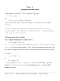
7 Notice that for this model (and indeed for anyGaussian posterior) themeanof the posterior distributionp(w|y,X) is alsoits mode, which is also called themaximum a posteriori(MAP) estimate ofMAP estimate2 Often Bayes rule is stated asp(a|b) =p(b|a)p(a)/p(b); here we use it in a form where weadditionally condition everywhere on the inputsX(but neglect this extra conditioning forthe prior which is independent of the inputs).C. E. Rasmussen & C. K. I. Williams, Gaussian Processes for Machine Learning , the MIT Press, 2006,ISBN 2006 Massachusetts Institute of , w1slope, w2 2 1012 2 1012 505 505input, xoutput, y(a)(b)intercept, w1slope, w2 2 1012 2 1012intercept, w1slope, w2 2 1012 2 1012(c)(d)Figure :Example of Bayesian linear modelf(x) =w1+w2xwith interceptw1and slope parameterw2. Panel (a) shows the contours of the prior distributionp(w) N(0, I), eq. ( ). Panel (b) shows three training points marked by (c) shows contours of the likelihoodp(y|X,w) eq.

8 ( ), assuming a noise level of n= 1; note that the slope is much more well determined than the intercept. Panel(d) shows the posterior,p(w|X,y) eq. ( ); comparing the maximum of the posteriorto the likelihood, we see that the intercept has been shrunk towards zero whereas themore well determined slope is almost unchanged. All contour plots give the 1 and2 standard deviation equi-probability contours. Superimposed on the data in panel(b) are the predictive mean plus/minus two standard deviations of the (noise-free)predictive distributionp(f |x , X,y), eq. ( ).w. In a non-Bayesian setting the negative log prior is sometimes thought ofas apenaltyterm, and the MAP point is known as the penalized maximumlikelihood estimate of the weights, and this may cause some confusion betweenthe two approaches. Note, however, that in the Bayesian setting the MAPestimate plays no special r penalized maximum likelihood procedure3In this case, due to symmetries in the model and posterior, it happens that the meanof the predictive distribution is the same as the prediction at the mean of the , this is not the case in E.

9 Rasmussen & C. K. I. Williams, Gaussian Processes for Machine Learning , the MIT Press, 2006,ISBN 2006 Massachusetts Institute of Weight-space View11is known in this case asridgeregression [Hoerl and Kennard, 1970] because ofridge regressionthe effect of the quadratic penalty term12w> 1pwfrom the log make predictions for a test case we average over all possible parameterpredictive distributionvalues, weighted by their posterior probability. This is in contrast to non-Bayesian schemes, where a single parameter is typically chosen by some crite-rion. Thus the predictive distribution forf ,f(x ) atx is given by averagingthe output of all possible linear models the Gaussian posteriorp(f |x ,X,y) = p(f |x ,w)p(w|X,y)dw=N(1 2nx> A 1Xy,x> A 1x ).( )The predictive distribution is again Gaussian , with a mean given by the poste-rior mean of the weights from eq. ( ) multiplied by the test input, as one wouldexpect from symmetry considerations. The predictive variance is a quadraticform of the test input with the posterior covariance matrix, showing that thepredictive uncertainties grow with the magnitude of the test input, as one wouldexpect for a linear example of Bayesian linear regression is given in Figure Here wehave chosen a 1-d input space so that the weight-space is two-dimensional andcan be easily visualized.

10 Contours of the Gaussian prior are shown in panel (a).The data are depicted as crosses in panel (b). This gives rise to the likelihoodshown in panel (c) and the posterior distribution in panel (d). The predictivedistribution and its error bars are also marked in panel (b). Projections of Inputs into Feature SpaceIn the previous section we reviewed the Bayesian linear model which suffersfrom limited expressiveness. A very simple idea to overcome this problem is tofirst project the inputs into some high dimensional space using a set of basisfeature spacefunctions and then apply the linear model in this space instead of directly onthe inputs themselves. For example, a scalar inputxcould be projected intothe space of powers ofx: (x) = (1,x,x2,x3,..)>to implement polynomialpolynomial regressionregression. As long as the projections are fixed functions ( independent ofthe parametersw) the model is still linear in the parameters, and thereforelinear in the parametersanalytically idea is also used in classification, where a datasetwhich is not linearly separable in the original data space may become linearlyseparable in a high dimensional feature space, see section Application ofthis idea begs the question of how to choose the basis functions?