Transcription of Hall Effect Experiment - University of Tennessee
1 Hall Effect Experiment by Dr. G. Bradley Armen Department of Physics and Astronomy 401 Nielsen Physics Building The University of Tennessee Knoxville, Tennessee 37996-1200 Copyright April 2007 by George Bradley Armen* *All rights are reserved. No part of this publication may be reproduced or transmitted in any form or by any means, electronic or mechanical, including photocopy, recording, or any information storage or retrieval system, without permission in writing from the author. 1. Introduction The Hall Effect is basic to solid-state physics and an important diagnostic tool for the characterization of materials particularly semi-conductors. It provides a direct determination of both the sign of the charge carriers, electron or holes (appendix A), and their density in a given sample.
2 The basic setup is shown in Fig. 1: A thin strip (thickness ) of the material to be studied is placed in a magnetic field B oriented at right angles to the strip. Fig. 1: Hall Effect geometry. This arrangement corresponds to our laboratory setup. A current I is arranged to flow through the strip from left to right, and the voltage difference between the top and bottom is measured. Assuming the voltmeter probes are vertically aligned, the voltage difference is zero when B = 0. The current I flows in response to an applied electric field, with its direction established by convention. However, on the microscopic scale I is the result of either positive charges moving in the direction of I, or negative charges moving backwards. In either case, the magnetic Lorentz force Bv q causes the carriers to curve upwards.
3 Since charge cannot leave the top or bottom of the strip, a vertical charge imbalance builds up in the strip. This charge imbalance produces a vertical electric field which counteracts the magnetic force, and a steady-state situation is reached. The vertical electric field can be measured as a transverse potential difference on the voltmeter. Suppose now that the charge carriers where electrons (eq =). In this case negative charge accumulates on the strip s top so the voltmeter would read a negative potential difference. Alternately, should the carriers be holes (eq+=) we measure a positive voltage. The above argument provides a simple picture in which to think about the Hall Effect and in fact leads to the correct answer if pursued. However, it presupposes a steady current of charge carriers flowing in the conductor all in a single direction with constant speed.
4 Why, for instance, don t the carriers accelerate? The true nature of macroscopic conduction is a bit more complicated, relying on a statistical average over individual carrier s motions. In the next section we will briefly look at this issue. 2. The Drude theory and the Hall Effect Before considering the Effect of magnetic fields on conductors, we need some model to describe the flow of currents in response to electric fields. To do so we will use the Drude theory of conductors. This is a simple classical model, and many of its concepts extend to the quantum case. A more careful account of the Drude model can be found in the first chapter of Solid State Physics by Ashcroft and Mermin. The Drude model envisions a conductor as a gas of free current-carrying charges.
5 The freely moving carriers suffer randomizing collision events on average every seconds. The parameter is called the relaxation time1, and is the only feature describing the (otherwise unspecified) collision events. Fig. 2: Example of a charge carrier s random trajectory after four collision events. Figure 2 indicates the basic idea. The solid black lines show a specific trajectory of a charge carrier in the absence of any external force. It proceeds with some constant 1 One might think that collisions occur more often the faster the particles are moving, so that could depend on the average particle velocity V. However, we ll see that the thermal velocities the carriers actually move with between collisions is very much greater than V.
6 Velocity in some direction until it experiences a thermal2 collision. The red dashed lines indicate how each of these trajectories would be influenced by a constant external force F: The particle now accelerates in the direction of F consistent with its initial conditions dictated by the last collision. When these paths are assembled, we see that F has caused a net displacement x after the four collisions; the particle has begun to drift in the direction of F. For macroscopic quantities, only averages over all particles are of interest. With the above assumptions, one can obtain an equation of motion for the average momentum P, given by FPP=+ 1dtd. Here, P is interpreted as follows: a group of charge carriers (say2310 ) all have some specific average momentum P0 at t = 0, the group s average momentum P(t) at any future time is then determined by this initial value and the first order equation above.
7 The average momentum P of the group evolves in time like a single carrier subjected to the average external force F per particle, but subjected additionally to a resistive damping. This damping is a consequence of all the random collisions; when is large collisions are uncommon. For a constant force a terminal momentum is reached independent of the initial conditions. This is in complete analogy with the motion of an object falling through air: the object either speeds up or slows down enough so that the air-resistance counteracts its weight. In our case P becomes constant in time as FP . Thus, if we apply a force F and wait long enough, a steady state develops where, on average, each particle drifts with a constant speed in the direction of F.
8 In response to a constant electric field (EFq=) a constant current of charge carriers is established. The current density J is the average charge crossing an (oriented) area per unit time. If there are n charge carriers per unit volume with average (drift) 2 That is, the new velocity has a random direction and its magnitude, unrelated to the old velocity, is consistent with the temperature at the collision site ( on average mv2 = kT ) velocity m/PV=, the associated current density is mqnqnq/EVJ ==. Thus, we arrive at Ohm s law JEEEJ = =or 2mnq, where is the conductivity, and /1= the resistivity, of the material; nqm2 =. Note that is inversely proportional to the relaxation time.
9 Since we expect that decreases with increasing temperature (carrier collisions occur more often), we expect a metal s resistance to increase with temperature (which it does). Now, consider what happens when we apply a magnetic field B to a thin strip of material in which a current I is flowing, as shown in Fig. 3. Fig. 3: Hall Effect geometry again; the strip has a thickness , length l, and height h. Here, the applied field B is directed only in the z direction (into the paper). The x-component of E drives the steady current I in the x direction, and a y-component of E must appear to balance the Lorentz force on the charge carriers: The equation of motion (in SI units) is []BVEVV +=+mqdtd 1. Again, when a steady current flow is established the time derivative of V at each point vanishes3.
10 Multiplying the above by qn , the time-independent result can be written in terms of J as ()BJEJ +=mq . With the setup shown in Fig. 3 steady current can only flow in the x directionxJ J=, while zB B=. Performing the cross product and resolving into components gives JBmqEJEyx == and . Along with Ohm s law describing current flow along the strip, we now have a component to the electric field in the transverse direction proportional to J and B. The Hall Coefficient (or Constant) RH is officially defined as this proportionality constant: JBREHy=. The Drude model thus predicts nqRH1=. The Hall constant thus gives a direct indication of the sign of the charge carriers; it is negative for electrons (eq =) and positive for holes (eq+=).