Transcription of Histogram Equalization - Home | UCI Mathematics
1 Histogram EqualizationHistogram Equalization is a technique for adjusting image intensities to enhance a given image represented as amrbymcmatrix of integer pixel intensities rangingfrom 0 toL the number of possible intensity values, often 256. Letpdenote thenormalized Histogram offwith a bin for each possible intensity. Sopn=number of pixels with intensityntotal number of pixelsn= 0,1, .., L Histogram equalized imagegwill be defined bygi,j= floor((L 1)fi,j n=0pn),(1)where floor() rounds down to the nearest integer. This is equivalent to transforming thepixel intensities,k, offby the functionT(k) = floor((L 1)k n=0pn).The motivation for this transformation comes from thinkingof the intensities offandgascontinuous random variablesX,Yon [0, L 1] withYdefined byY=T(X) = (L 1) X0pX(x)dx,(2)wherepXis the probability density function the cumulative distributive functionofXmultiplied by (L 1). Assume for simplicity thatTis differentiable and invertible.
2 Itcan then be shown thatYdefined byT(X) is uniformly distributed on [0, L 1], namelythatpY(y) =1L 1. y0pY(z)dz= probability that 0 Y y= probability that 0 X T 1(y)= T 1(y)0pX(w)dwddy( y0pY(z)dz)=pY(y) =pX(T 1(y))ddy(T 1(y)).1original histogramtransformed histogramFigure 1: Histogram Equalization applied to low contrast imageNote thatddyT(T 1(y)) =ddyy= 1, sodTdx|x=T 1(y)ddy(T 1(y)) = (L 1)pX(T 1(y))ddy(T 1(y)) = 1,which meanspY(y) =1L discrete Histogram is an approximation ofpX(x) and the transformation in Equation1 approximates the one in Equation 2. While the discrete version won t result in exactlyflat histograms, it will flatten them and in doing so enhance the contrast in the image. Theresult of applying Equation 1 to the test image is shown in Figure :To test the accompanying code, , typeg = hist_eq( ); Histogram Equalization is also built into MATLAB. Type2help histeqto see how it :What happens if Equation 1 is applied twice?
3 Reference:R. C. Gonzalez and R. E. Woods,Digital Image Processing, Third Edition.