Transcription of How to combine errors
1 How to combine errors 400. Robin Hogan Blackbody irradiance (W m 2). June 2006. 300. 1 What is an error ? F + F. All measurements have uncertainties that need to 200. be communicated along with the measurement itself.. F. Suppose we make a measurement of temperature, T , F. T. but the true temperature is T . In this case our instan- 100. taneous error is T = T T . Obviously we don't know the value of T for any specific measurement T T+ . T. (otherwise we could simply subtract it and report the 0. 0 100 200 300.)
2 True value) but we should be able to estimate the root- Temperature (K). mean-squared error, given by Figure 1: Illustration of the estimation of the error in F. from the error in T using the gradient of the relationship q T = 2T , (1) between them (using Eq. 2). and then report our measurement in the form T T. (for example T = K). In Eq. 1, the overbar in which we use the definition of an error in Eq. 1 to denotes the mean taken over a large number of mea- estimate the error in the new variable given the errors surements by an identical instrument.
3 In the measured variables. However, if only one mea- Usually the quantity T is referred to simply as surement is involved then we can use a simpler method the error in the measurement . This is a bit mislead- based on differentiation. ing and is easy to confuse with the instantaneous error; Suppose we wish to derive the irradiance F emit- a better term would have been uncertainty , but er- ted by a blackbody with a temperature T using ror is in such common use that we had better stick with it. Just keep in mind that what we usually mean F = T 4 , (2).
4 Is the root-mean-squared error. If the instantaneous errors have a Gaussian distri- where is a constant that is known very accurately. It bution (also known as a Normal or Bell-shaped distri- can be seen from Fig. 1 that, provided the error in T. bution) then approximately 68% of the individual mea- is relatively small, the ratio of instantaneous errors in surements will lie between T T and T + T , and F and T is approximately equal to the gradient of the 95% of them between T 2 T and T +2 T . Be aware relationship between them: that sometimes errors are stated to indicate the 95% F dF.
5 Confidence interval , in which case they are equal to . (3). T dT. 2 T . It should be noted that the measurement may well be the mean of a number of samples, in which From now on we will replace with = , but al- case we might take the standard error of the mean as ways be aware that error estimation is an approximate an estimate of the error T . business so it is not worth quoting errors to high preci- sion (certainly no more than two significant figures). 2 errors for functions of one variable With the help of Eq.
6 1, it can be shown that the ratio of root-mean-squared errors is Usually we will have a formula we want to use to derive a new variable from one or more of our mea- F F dF. sured variables. Section 3 describes the general case = = , (4). T T dT. 1. where | | denotes the absolute value ( removing The term b c is an error covariance and is zero pro- any minus sign) and is present because the root-mean- vided that the measurements independent, their in- square of a real number is always positive. If we mea- stantaneous errors are uncorrelated.
7 Thus for indepen- sure the temperature to be T T then we can use Eq. dent measurements of b and c, the error formula is 4 to obtain the error in F: q a = ( b)2 + ( c)2 . (11). dF. F = T = 4 T 3 T . (5). dT The error formulae for addition, subtraction, multipli- In the general case of a formula of the form a = cation and division of independent variables can be de- f (b), the error in a is given by rived in a similar manner: Functions of more than one variable d f (b). a = b. (6) ). db a=b+c ( a)2 = ( b)2 + ( c)2.
8 The error formulae for some common functions have a=b c been calculated using Eq. 6 and are given below a b c ) 2 2 2. a = bc . (where a and b are variables and and are constants): = +. a = b/c a b c Functions of one variable a = b+c+d ( a)2 = ( b)2 + ( c)2 + ( d)2. a = b a = | | b a = bcd ( a/a)2 = ( b/b)2 + ( c/c)2. a = /b a = /b2 b = |a/b| b + ( d/d)2. a = b a = b 1 b = | a/b| b (12). a = exp( b) a = | a| b a = ln( b) a = | /b| b 4 errors for more complicated formulae (7). For more complicated formulae we can combine the 3 Functions of two or more variables approaches in sections 2 and 3.
9 For example, consider the formula In the general case, the quantity we want to calcu- a = b exp(c). (13). late depends on more than one measurement , a =. f (b, c, ..), and a more rigorous approach is needed to If we let a = xy where x = b and y = exp(c), work out how the error in a depends on the errors in the then from Eq. 7 we know that x = | x/b| b and other variables. Taking the simplest possible formula y = |y| c. According to Eq. 12, we can combine these errors using the multiplication rule to obtain a = b + c, (8).
10 A x 2 y 2. 2 . = +. we replace a by a + a , etc., to obtain a + a = b + b + a x y c + c . Noting that a = b + c , the relationship between . b 2. the instantaneous errors is then simply = + ( c)2 . (14). b a = b + c . (9) and hence " 2 #1. From the definition of an error given in Eq. 1 we have b 2. a = a + ( c)2 . (15). q q b a = 2a = ( b + c )2. q = 2b + 2c + 2 b c q = ( b)2 + ( c)2 + 2 b c . (10). 2.