Transcription of How to Graph Point Estimates and 95% Confidence …
1 Biostatistics Graphing Confidence Intervals 1 2009 Johns Hopkins University Department of Biostatistics 10/01/09 How to Graph Point Estimates and 95% Confidence Intervals Using Stata 11 or Excel The methods presented here are just several of many ways to construct the Graph . A. Simplest method using Stata: One simple way in which to portray a graphical representation of the Confidence intervals for the difference in mean weight change for each of the age-gender groups is to use the Stata command serrbar, with the option scale( ) to provide bars extending to +/- standard errors. 1) First, create a new small data set in the editor by manually entering the following variables: agegen (age-gender group), mean(the mean weight change within an age-gender group), and se (the associated standard error of the mean weight change).
2 Enter the following values into the Stata data editor: . list agegen mean se 1. 1 2. 2 3. 3 4. 4 2) Label the agegen variable: . label define agegen 1 "M < 30" 2 "M 30+" 3 "F < 30" 4 "F 30+" . label values agegen agegen . list agegen mean se 1. M < 30 2. M 30+ 3. F < 30 4. F 30+ Biostatistics Graphing Confidence Intervals 2 2009 Johns Hopkins University Department of Biostatistics 10/01/09 3) Graph using the serrbar command: . serrbar mean se agegen, scale ( ) 0102030mean1234agegen 4) Enhance the serrbar command with some options: serrbar mean se agegen, scale ( ) title("95% Confidence Interval for Mean Weight Change") sub("Between Current Weight and Weight at Age 18") yline(0) yline(0) b2(Age-Gender Group) t1(95% Confidence Interval for Mean Weight Change) l1(Weight Change (pounds)) ylab(-5(5)35) xlab(1(1)4) xlabel(, valuelabel) -505101520253035meanM < 30M 30+F < 30F 30+agegenWeight Change (pounds)95% Confidence Interval for Mean Weight ChangeAge-Gender GroupBetween Current Weight and Weight at Age 1895% Confidence Interval for Mean Weight ChangeBiostatistics Graphing Confidence Intervals 3 2009 Johns Hopkins University Department of Biostatistics 10/01/09 B.
3 Method 2 using Stata: 1) Enter the data as follows, with a separate line for the lower limit of the CI, the mean, and the upper limit of the CI: group level change 1 Lower 1 Mean 1 Upper 2 Lower 2 Mean 2 Upper 3 Lower 3 Mean 3 Upper 4 Lower 4 Mean 4 Upper 2) Label the age-gender group variable. label define agegenf 1 "M < 30" 2 "M 30+" 3 "F < 30" 4 "F 30+" label values group agegenf 3) Sort the data. egen xmin=min(group), by(group) egen xmax=max(group), by(group) gsort -xmin -xmax group group 4) Plot using the twoway scatter command. twoway scatter change group, msymbol(+) c(L) xlab(1(1)4) ylab(-5(5)35) l2("95% Confidence Interval") l1("for the true mean change in weight") b2(Age-Gender Group) t1(Example of Graph comparing 95% Confidence intervals) yline(0) xlabel(, valuelabel) 5) The above commands yield the following plot: -505101520253035 ChangeM < 30M 30+F < 30F 30+Groupfor the true mean change in weight95% Confidence IntervalExample of Graph comparing 95% Confidence intervalsAge-Gender Group Biostatistics Graphing Confidence Intervals 4 2009 Johns Hopkins University Department of Biostatistics 10/01/09 C.
4 A method using Excel: Step 1: Enter the data into a new spreadsheet. You will need to enter the group variable, the mean and the error bound (this is the critical value (t or z) times the standard error, aka the difference from the mean to the Confidence limits). For our example, enter the data as illustrated below: Group Mean ErrorBound 1 2 7 3 4 Step 2: Follow the steps below using the Chart Wizard to construct the Graph . a) Using the mouse, select the Group and Mean values. b) Click on the Chart Wizard . c) Select XY (Scatter) , click Next . d) Select: Series in Columns, click Next . e) Remove Gridlines, add axis labels as you want, click Next . f) Select how you want to store the Graph , click Finish.
5 G) Go into the Graph and double-click on one of the data points. h) A menu will appear titled Format Data Series . i) Select Y Error Bars menu. j) In Display , select Both . k) In Error Amount , select Custom . l) You want to add and subtract the error bounds that you entered into the spreadsheet, so for each + and - , select the error bounds from your spreadsheet by click and dragging over these values. m) Then select Okay . The Graph you obtain looks something like this: Example of 95% Confidence intervalsM,<30M,30+F,<30F,30+05101520253 035 Group95% Confidence interval for the true mean difference in weight You may want to change the labels for the groups or axis labels or title.