Transcription of Introduction of Particle Image Velocimetry - UMD
1 Introduction of Particle Image VelocimetrySlides largely generated by J. Westerweel & C. Poelma of Technical University of DelftAdapted by K. KigerKen KigerBurgers Program For Fluid DynamicsTurbulence SchoolCollege Park, Maryland, May 24-27 IntroductionParticle Image Velocimetry (PIV):Imaging of tracer particles , calculate displacement: local fluid velocityTwin Nd:YAGlaserCCD cameraLight sheetopticsFrame 1: t = t0 Frame 2: t= t0+ tMeasurementsectionIntroductionParticle Image Velocimetry (PIV)99210043232 divide Image pair ininterrogation regions small region:~ uniform motion compute displacement repeat !!!IntroductionParticle Image Velocimetry (PIV):Instantaneous measurement of 2 components in a planeconventional methods(HWA, LDV) single-point measurement traversing of flow domain time consuming only turbulence statisticszparticle Image Velocimetry whole-field method non-intrusive (seeding instantaneous flow fieldIntroductionParticle Image Velocimetry (PIV):Instantaneous measurement of 2 components in a planeparticle Image Velocimetry whole-field method non-intrusive (seeding instantaneous flow fieldinstantaneous vorticity fieldExample: coherent structuresExample: coherent structuresTurbulent pipe flowRe= 5300100 85 vectors hairpin vortexExample: coherent structuresVan Doorne, et components.))
2 - tracer particles - light source- light sheet optics- camera- measurement settings- interrogation- post-processingHardware (imaging)Software ( Image analysis)Tracer particlesAssumptions:- homogeneously distributed- follow flow perfectly- uniform displacement within interrogation regionCriteria:-easily visible- particles should not influence fluid flow!small, volume fraction < 10-4 Image densityNI<< 1NI>> 1particle tracking velocimetryparticle Image velocimetrylow Image densityhigh Image densityAssumption: uniform flow in interrogation area Evaluation at higher densityHigh NI : no longer possible/desirable to follow individual tracer particlesParticle can be matched with a number of candidatesPossible matches Repeat process for other particles , sum up: wrong combinations will lead to noise, but true displacement will dominateSum of all possibilitiesStatistical estimate of Particle motion Statistical correlations used to find average Particle displacement1-d Image @ t=t01-d Image @ t=t1R(i,j)Ia(k,l)I aIb(ki,lj)I bl1 Byk1 BxIa(k,l)I a2Ib(ki,lj)I b2l1 Byk1 Bxl1 Byk1Bx12xyBkBlayxalkIBBI1 1),(1 Cross-correlation1-D cross-correlation exampleR(i)Ia(k)I aIb(ki)I bk1 BxIa(k)I a2Ib(ki)I b2k1 Bxk1Bx12 IaIbIa(x) normalizedIb(x+x) normalizedIa(x)*Ib(x+x)Finding the maximum displacement-Shift 2ndwindow with respect to the first- Calculate match - Repeat to find best estimateTypically 16x16 or 32x32 pixelsGood indicator:R(i,j)Ia(k,l)I aIb(ki,lj)I bl1 Byk1 BxIa(k,l)I a2Ib(ki,lj)I b2l1 Byk1 Bxl1 Byk1Bx12xyBkBlayxalkIBBI1 1),(1 Finding the maximum displacementBad match.
3 Sum of product of intensities low-Shift 2ndwindow with respect to the first- Calculate match - Repeat to find best estimateTypically 16x16 or 32x32 pixelsGood indicator:R(i,j)Ia(k,l)I aIb(ki,lj)I bl1 Byk1 BxIa(k,l)I a2Ib(ki,lj)I b2l1 Byk1 Bxl1 Byk1Bx12xyBkBlayxalkIBBI1 1),(1 Finding the maximum displacementGood match: sum of product of intensities high-Shift 2ndwindow with respect to the first- Calculate match - Repeat to find best estimate Can be implemented as 2D FFT for digitized dataoImpose periodic conditions on interrogation bias error if not treated 16x16 or 32x32 pixelsGood indicator:R(i,j)Ia(k,l)I aIb(ki,lj)I bl1 Byk1 BxIa(k,l)I a2Ib(ki,lj)I b2l1 Byk1 Bxl1 Byk1Bx12xyBkBlayxalkIBBI1 1),(1 Cross-correlationThis shifting method can formally be expressed as a cross-correlation:12()RIIdsxx sx- I1and I2are interrogation areas (sub-windows) of the total frames- x is interrogation location- s is the shift between the images Backbone of PIV:-cross-correlation of interrogation areas-find location of displacement peakCross-correlationRDRFRC correlation of the meancorrelation of mean & random fluctuationscorrelation due to displacementpeak: meandisplacementInfluence of NINI= 5NI= 10NI= 25 More particles : better signal-to-noise ratioUnambiguous detection of peak from noise:NI=10 (average), minimum of 4 per area in 95% of areas(number of tracer particles is a Poisson distribution)RNNC zMDDDIII( ) ~s0022 Cparticle concentrationz0light sheet thicknessDIint.
4 Area sizeM0magnificationInfluence of NINI= 5NI= 10NI= 25 PTV: 1 Particle used for velocity estimate; error ePIV: error ~ e/sqrt(NI)Influence of in-plane displacementX / DI = ),(~)(sX,Y-Displacement<quarter of window sizeInfluence of out-of-plane displacementZ / z0 = F FF zzzDDI I OO( ) ~()s10Z-Displacement<quarter of light sheet thickness(z0)Influence of gradientsDisplacement differences <3-5% of int. area size, DIDisplacement differences < Particle Image size, da / DI = / d= F F FF aa dDDI I O( ) ~( )exp(/)s22a Keane & AdrianPIV Design rules Image densityNI>10 in-plane motion|X| < DI out-of-plane motion |z| < z0 spatial gradientsM0ut< dObtained by Keane & Adrian (1993) using synthetic dataWindow shifting in-plane motion|X| < DIstrongly limits dynamic range of PIVlarge window size: too much spatial averagingWindow shifting in-plane motion|X| < DIstrongly limits dynamic range of PIVsmall window size: too much in-plane pair lossWindow shifting in-plane motion|X| < DIstrongly limits dynamic range of PIVM ulti-pass approach:start with large windows,use this result as pre-shift for smaller more in-plane pair loss limitations!
5 Window shifting: Examplefixed windowsmatched windowsGrid turbulencewindows at same locationwindows at 7px downstream Window shifting: ExampleVortex ring, decreasing window sizesRaffel,Willert andKompenhansSub-pixel accuracyMaximum in the correlation plane: single-pixel resolution of displacement?But the peak contains a lot more information!Gaussian Particle images Gaussian correlation peak (but smeared)Sub-pixel accuracyFractional displacement can be obtained using the distribution of gray values around maximumr X peak centroid parabolic peak fit Gaussian peak fitRRRRR11101 RRRRR1111022lnlnlnlnlnRRRRR1111022balanc enormalizationthree-point estimatorsPeak locking zig-zag structure, sudden kinks in the flowSub-pixel Interpolation Errors Accuracy depends on: Particle Image size noise in data (seeding density, camera noise) shear rate Can exhibit peak locking Interpolation of peak is biased towards a symmetric data distribution (Integer and 1/2 integer peak locations) Polynomials exhibit strong locking when Particle diameter is small Gaussian is most commonly used Splines are very robust, but expensive to calculate See Particle Image Velocimetry , by Raffel, Willert, and Kompenhans, Springer-Verlag, peak location (pixels)Interpolation error (pixels)Polynomial fitGaussian peak location (pixels)Interpolation error (pixels)Polynomial fitGaussian peak location (pixels)Interpolation error (pixels)Polynomial fitGaussian fitR = = = RadiusPeak lockingcentroidGaussian peak fitEven with Gaussian peak fit.
6 Particle Image size too small peak locking(Consider a point Particle sampled by discrete pixels)Histogram of velocities in a turbulent flowSub-pixel accuracyoptimal resolution: Particle Image size: ~2 pxSmaller: Particle no longer resolvedLarger: random noise increase three-point estimators:Peak centroidParabolic peak fitGaussian peak difference: sensitivity to peak locking or pixel lock-in , bias towards integer displacementsTheoretical: pxIn practice pxbias errorsrandom errorstotalerrord/ drdisplacement measurement errorfixed windowsmatched windowssignalnoiseSNRu 2C2u 2 / C2u 24C2u 21 / 4C2FI~ ~ 1velocity pdfmeasurementerrorwindow matchingfixed windowsmatched windowsX= 7 pxu /U = example:grid-generated turbulenceData Validation article lab Spurious or Bad vectorsSpurious vectorsThree main causes:-insufficient Particle - Image pairs-in-plane loss-of-pairs, out-of-plane loss-of-pairs-gradientsEffect of tracer densityNI= 1NI= 3NI= 5NI=11NI=20NI=45NI=80 Remedies increase NI practical limitations: optical transparency of the fluid two-phase effects Image saturation / speckle detection, removal & replacement keep finite NI( ~ ) data loss is small signal loss occurs in isolated points data recovery by interpolationDetection methods human perception peak height amount of correlated signal peak detectability peak height relative to noise lower limit for SNR residual vector analysis fluctuation of displacement multiplication of correlation planes fluid mechanics continuity fuzzy logic & neural netsResidual analysis evaluate fluctuation of measured velocity residual ideally: Uref= true velocity reference values.
7 Uref= global mean velocity comparable to 2D-histogram analysis does not take local coherent motion into account probably only works in homogeneous turbulence Uref= local (3 3) mean velocity takes local coherent motion into account very sensitive to outliers in the local neighborhood Uref= local (3 3) median velocity almost identical statistical properties as local mean Strongly suppressed sensitivity to outliers in heighborhoodrefUUrExample of residual mean and are very sensitive to bad data need robust measure of fluctuationMedian test1234056781 - Calculate reference velocity: median of 8 neighbors2 calculate residuals:3 Normalize target residual by: median(ri) + 4 Robust measure found for:urefmedian u1,u2.
8 U8riuiurefr0*u0urefmedian(ri) and r0*2 Westerweel & Scarano, 2005 InterpolationBilinear interpolation satisfies continuityFor 5% bad vectors, 80% of the vectors are isolatedBad vector can be recovered without any : interpolation biases statistics (power spectra, correlation function)Better not to replace bad vectors (use slotting method)Overlapping windowsMethod to increase data yield:Allow overlap between adjacent interrogation areasaMotivation: Particle pairs near edgescontribute less to correlation result;Shift window so they are in the center:additional, relatively uncorrelated result50% is very common, but beware of oversamplingA Generic PIV programData acquisitionImage pre-processingPIV cross-correlationVector validationPost-processingLaser control,Camera settings, non-uniformityof illumination; ReflectionsPre-shift; Decreasingwindow sizesVorticity, interpolationof missing vectors, test,Search windowPIV softwareFreePIVware: command line, linux (Westerweel)JPIV: Java version of PIVware (Vennemann)MatPiv: Matlab PIV toolbox (Cambridge, Sveen)URAPIV: Matlab PIV toolbox (Gurka and Liberzon)DigiFlow (Cambridge), PIV Sleuth (UIUC), MPIV, GPIV, CIV, OSIV.
9 CommercialPIVtecPIVviewTSII nsightDantecFlowmapLaVisionDaVisOxford Motion: tracer Particle Equation of motion for spherical Particle : Where Neglect: non-linear drag (only really needed for high-speed flows), Basset history term (higher order effect)gmdtudmdtvddtudmvuDdtvdmpgpfpfppp 1213mppD36, the Particle massmffD36, fluid mass of same volume as particleD Particle diameter fluid viscosityr u fluid velocityr v p Particle velocityg fluid densityp Particle material densityAdded massViscous dragPressure gradientbuoyancyInertiaSimple thought experiment Lets see how a Particle responds to a step change in velocity Only consider viscous dragmpdr v pdt3Dr u r v pu0 for t< 0U for t0dvpdt18pD2 Uvp1pUvpvpvpparticularvphomogeneousUC1ex ptpv p1pvp1pUvpU1exptpu, vptUParticle Transfer Function Useful to examine steady-state Particle response to 1-D oscillating flow of arbitrary sum of frequencies Represent u as an infinite sum of harmonic functions Neglect gravity (DC response, not transient)
10 U tf0expitdvptp0expitd2mp3 Ddvpdt2uvpmfmpmp3 Ddudtdvpdt2mfmpmp3 Ddudtdutdtif0expitd2pD218piexpit0d2fpexp it0dfppD218i3fpexpitd02iStp2fpiSt3fpdvpt dtip0expitdStpfpD218 fpParticle Transfer Function This can be rearranged: Examine Liquid in air, gas in water, plastic in waterr v pr u ppff1 2A2B2A211 22322 BStAtan1 Imp/fRep/ftan1A(1B)A2 BLiquid particles in Air Liquid drops in air require St~ for 95% fidelity (1 m ~ 15 kHz) Size relatively unimportant for near-neutrally buoyant particles Bubbles are a poor choice: always overrespond unless quite small