Transcription of Introduction to Binary Logistic Regression
1 Introduction to Binary Logistic Regression 1 Introduction to Binary Logistic Regression Dale Berger Email: Website: Page Contents 2 How does Logistic Regression differ from ordinary linear Regression ? 3 Introduction to the mathematics of Logistic Regression 4 How well does a model fit? Limitations 4 Comparison of Binary Logistic Regression with other analyses 5 Data screening 6 One dichotomous predictor: 6 Chi-square analysis (2x2) with Crosstabs 8 Binary Logistic Regression 11 One continuous predictor: 11 t-test for independent groups 12 Binary Logistic Regression 15 One categorical predictor (more than two groups) 15 Chi-square analysis (2x4) with Crosstabs 17 Binary Logistic Regression 21 Hierarchical Binary Logistic Regression w/ continuous and categorical predictors 23 Predicting outcomes, p(Y=1) for individual cases 24 Data source, reference, presenting results 25 Sample results.
2 Write-up and table 26 How to graph Logistic models with Excel 27 Plot of actual data for comparison to model 28 How to graph Logistic models with SPSS 1607 Introduction to Binary Logistic Regression 2 How does Logistic Regression differ from ordinary linear Regression ? Binary Logistic Regression is useful where the dependent variable is dichotomous ( , succeed/fail, live/die, graduate/dropout, vote for A or B). For example, we may be interested in predicting the likelihood that a new case will be in one of the two outcome categories. Why not just use ordinary Regression ? The model for ordinary linear Regression (OLS) is Yi = Bo + B1Xi + errori Suppose we are interested in predicting the likelihood that an individual is a female based on body weight.
3 Using real data from 190 Californians who responded to a survey of licensed drivers (Berger et al., 1990), we could use WEIGHT to predict SEX (coded male = 0, female = 1). An ordinary least squares Regression analysis tells us that Predicted SEX = - .01016 * (Body Weight) and r = , t(188) = , p < .001. A na ve interpretation is that we have a great model. It is always a good idea to graph data to make sure models are appropriate. A scatter plot gives us intraocular trauma! The linear Regression model clearly is not appropriate. The test of statistical significance is based on the assumption that residuals from the Regression line are normally distributed with equal variance for all values of the predictor.
4 Clearly, this assumption is violated. The tests of statistical significance provided by the standard OLS analysis are erroneous. A more appropriate model would produce an estimate of the population average of Y for each value of X. In our example, the population mean approachs SEX=1 for smaller values of WEIGHT and it approaches SEX=0 for larger values of WEIGHT. As shown in the next figure, this plot of means is a curved line. This is what a Logistic Regression model looks like. It clearly fits the data better than a straight line when the Y variable takes on only two values. BODY WEIGHT OF RESPONDENT30025020015010050 Sex M=0 F = predicted SEX 100 150 .557 200 .049 250 For someone who weighs 150 pounds, the predicted value for SEX is.
5 557. Naively, one might interpret predicted SEX as the probability that the person is a female. However, the model can give predicted values that exceed and or are less than zero, so the predicted values are not probabilities. Introduction to Binary Logistic Regression 3 Introduction to the mathematics of Logistic Regression Logistic Regression forms this model by creating a new dependent variable, the logit(P). If P is the probability of a 1 at for given value of X, the odds of a 1 vs. a 0 at any value for X are P/(1-P). The logit(P) is the natural log of this odds ratio. Definition : Logit(P) = ln[P/(1-P)] = ln(odds). This looks ugly, but it leads to a beautiful model.
6 In Logistic Regression , we solve for logit(P) = a + b X, where logit(P) is a linear function of X, very much like ordinary Regression solving for Y. With a little algebra, we can solve for P, beginning with the equation ln[P/(1-P)] = a + b Xi = Ui. We can raise each side to the power of e, the base of the natural log, This gives us P/(1-P) = ea + bX. Solving for P, we get the following useful equation: bXabXaeeP 1 Maximum likelihood procedures are used to find the a and b coefficients. This equation comes in handy because when we have solved for a and b, we can compute P. This equation generates the curved function shown above, predicting P as a function of X. Using this equation, note that as a + bX approaches negative infinity, the numerator in the formula for P approaches zero, so P approaches zero.
7 When a + bX approaches positive infinity, P approaches one. Thus, the function is bounded by 0 and 1 which are the limits for P. Logistic Regression also produces a likelihood function [-2 Log Likelihood]. With two hierarchical models, where a variable or set of variables is added to Model 1 to produce Model 2, the contribution of individual variables or sets of variables can be tested in context by finding the difference between the [-2 Log Likelihood] values. This difference is distributed as chi-square with df= (the number of predictors added). The Wald statistic can be used to test the contribution of individual variables or sets of variables in a model. Wald is distributed according to chi-square. BODY WEIGHT OF RESPONDENT30025020015010050 Sex M=0 F = Introduction to Binary Logistic Regression 4 How well does a model fit?
8 The most common measure is the Model Chi-square, which can be tested for statistical significance. This is an omnibus test of all of the variables in the model. Note that the chi-square statistic is not a measure of effect size, but rather a test of statistical significance. Larger data sets will generally give larger chi-square statistics and more highly statistically significant findings than smaller data sets from the same population. A second type of measure is the percent of cases correctly classified. Be aware that this number can easily be misleading. In a case where 90% of the cases are in Group(0), we can easily attain 90% accuracy by classifying everyone into that group. Also, the classification formula is based on the observed data in the sample, and it may not work as well on new data.
9 Finally, classifications depend on what percentage of cases is assumed to be in Group 0 vs. Group 1. Thus, a report of classification accuracy needs to be examined carefully to determine what it means. A third type of measure of model fit is a pseudo R squared. The goal here is to have a measure similar to R squared in ordinary linear multiple Regression . For example, pseudo R squared statistics developed by Cox & Snell and by Nagelkerke range from 0 to 1, but they are not proportion of variance explained. Limitations Logistic Regression does not require multivariate normal distributions, but it does require random independent sampling, and linearity between X and the logit. The model is likely to be most accurate near the middle of the distributions and less accurate toward the extremes.
10 Although one can estimate P(Y=1) for any combination of values, perhaps not all combinations actually exist in the population. Models can be distorted if important variables are left out. It is easy to test the contribution of additional variables using hierarchical analyses. However, adding irrelevant variables may dilute the effects of more interesting variables. Multicollinearity will not produce biased estimates, but as in ordinary Regression , standard errors for coefficients become larger and the unique contribution of overlapping variables may become very small and hard to detect statistically. More data is better. Models can be unstable when samples are small. Watch for outliers that can distort relationships.