Transcription of Introduction to Gaussian Processes
1 Introduction to Gaussian ProcessesIain Introduction to Machine Learning, Fall 2008 Dept. Computer Science, University of TorontoThe problemLearn scalar function of vector valuesf(x) 1 f(x) 505x2x1fWe have (possibly noisy) observations{xi,yi}ni=1 Example ApplicationsReal-valued regression: Robotics: target state required torque Process engineering: predicting yield Surrogate surfaces for optimization or simulationClassification: Recognition: handwritten digits on cheques Filtering: fraud, interesting science, disease screeningOrdinal regression: User ratings ( movies or restaurants) Disease screening ( predicting Gleason score)Model complexityThe world is often 1 1 1 fitcomplex fittruthProblems: Fitting complicated models can be hard How do we find an appropriate model? How do we avoid over-fitting some aspects of model?Predicting yieldFactory settingsx1 profit of32 5monetary unitsFactory settingsx2 profit of100 200monetary unitsWhich are the best settingsx1orx2?
2 Knowing the error bars can be very high dimensions it takes many function evaluations tobe certain everywhere. Costly if experiments are 1 bars are needed to see if a region is still modellingIf we come up with a parametric family of functions,f(x; )and define a prior over , probability theory tells ushow to make predictions given data. For flexible models,this usually involves intractable integrals over .We re really good at integrating Gaussians though 2 1012 2 1012 Can we really solve significantmachine learning problems witha simple multivariate Gaussiandistribution? Gaussian distributionsCompletely described by parameters and :P(f| , ) =|2 | 12exp( 12(f )T 1(f )) and are the mean and covariance of the example: ij= fifj i jIf we know a distribution is Gaussian and know its meanand covariances, we know its density of GaussianThe marginal of a Gaussian distribution is (f,g) =N([ab],[A CC>B])As soon as you convince yourself that the marginalP(f) = dgP(f,g)is Gaussian , you already know the means and covariances:P(f) =N(a,A).
3 Conditional of GaussianAny conditional of a Gaussian distribution is also Gaussian :P(f,g) =N([ab],[A CC>B])P(f|g) =N(a+CB 1(y b), A CB 1C>)Showing this is not completely it is a standard result, easily looked observationsPreviously we if we only saw a noisy observation,y N(g,S)?P(f,g,y) =P(f,g)P(y|g)is Gaussian distributed; still aquadratic form inside the exponential after posterior overfis still Gaussian :P(f|y) dgP(f,g,y)(RHS is Gaussian after marginalizing, so still a quadraticform infinside an exponential.)Laying out GaussiansA way of visualizing draws from a 2D Gaussian : 2 1012 2 1012f1f2 x_1x_2 1 it s easy to show three drawsfrom a 6D Gaussian :x_1x_2x_3x_4x_5x_6 1 large GaussiansThree draws from a 25D Gaussian : 1012fxTo produce this, we needed a mean: I usedzeros(25,1)The covariances were set using akernelfunction: ij=k(xi,xj).Thex s are the positions that I planted the tics on the we ll findk s that ensure is always positive regression 1 1 GPf N(0,K), Kij=k(xi,xj)wherefi=f(xi)Noisy observations:yi|fi N(fi, 2n)GP PosteriorOur prior over observations and targets is Gaussian :P([yf ])=N(0,[K(X,X) + 2nIK(X,X )K(X ,X)K(X ,X )])Using the rule for conditionals,P(f |y)is Gaussian with:mean, f =K(X ,X)(K(X ,X) + 2nI) 1ycov(f ) =K(X ,X ) K(X ,X)(K(X,X) + 2nI) 1K(X,X )The posterior over functions is a Gaussian posteriorTwo (incomplete) ways of visualizing what we 1 1 p(f|data)Mean and error barsPoint predictionsConditional at one pointx is a simple Gaussian :p(f(x )|data) =N(m,s2)Need covariances:Kij=k(xi,xj),(k )i=k(x ,xi)Special case of joint posterior:M=K+ 2nIm=k> M 1ys2=k(x ,x ) k> M 1k positiveDiscovery or prediction?
4 What should error-bars show? 1 * 2 , p(y*|data) 2 , p(f*|data)True fPosterior MeanObservationsP(f |data) =N(m,s2)says what we know about thenoiseless (y |data) =N(m,s2+ 2n)predicts what we ll see so farWe can represent a function as abigvectorfWe assume that this unknown vector was drawn from abigcorrelated Gaussian distribution, aGaussian process.(This might upset some mathematicians, but for all practical machine learning and statistical problems, this is fine.)Observing elements of the vector (optionally corruptedby Gaussian noise) creates a posterior distribution. Thisis also Gaussian : the posterior over functions is still aGaussian marginalization in Gaussians is trivial, we caneasily ignore all of the positionsxithat are neither observednor functionsThe main part that has been missing so far is where thecovariance functionk(xi,xj)comes , other than making nearby points covary, what canwe express with covariance functions, and what do do theymean?
5 Covariance functionsWe can construct covariance functions from parametric modelsSimplest example:Bayesian linear regression:f(xi) =w>xi+b,w N(0, 2wI), b N(0, 2b)cov(fi,fj) = fifj >0 fi >0 fj = (w>xi+b)>(w>xj+b) = 2wx>ixj+ 2b=k(xi,xj)Kernel parameters 2wand 2barehyper-parametersin the Bayesianhierarchical interesting kernels come from models with a large or infinitefeature space. Because feature weightsware integrated out, this iscomputationally no more kernelAn number of radial-basis functions can givek(xi,xj) = 2fexp( 12D d=1(xd,i xd,j)2/`2d),the most commonly-used kernel in machine looks like an (unnormalized) Gaussian , so is commonlycalled the Gaussian that this hasnothing to do with it being Gaussian process need not use the Gaussian kernel. In fact, other choices will often be of hyper-parametersMany kernels have similar types of parameters:k(xi,xj) = 2fexp( 12D d=1(xd,i xd,j)2/`2d),Considerxi=xj, marginal function variance is 30 20 1001020 f = 2 f = 10 Meaning of hyper-parametersThe`dparameters give the overall lengthscale indimension-dk(xi,xj) = 2fexp( 12D d=1(xd,i xd,j)2/`2d),Typical distance between peaks ` 3 2 1012 l = = GP lengthscalesWhat is the covariance matrix like?
6 Consider 1D * , xoutput, * , 1 , x Zeros in the covariance would marginal independence Short length scales usually don t match my beliefs Empirically, I often learn` 1 giving a denseKCommon exceptions:Time series data,`small. Irrelevant dimensions,` high dimensions, can haveKij 0with` GPs are notLocally-Weighted Regression weights points with a kernelbefore fitting a simple * , xoutput, yx*kernel valueMeaning of kernel zero here: GP kernel:a) shrinks to small`with many datapoints; b) does not need to be positive of hyper-parametersDifferent (SE) kernel parameters give different explanationsof the 1 1 `= , n= `= , n= kernelsThe squared-exponential kernel some problems the Mat ern covariancesfunctions may be more appropriate:Periodic kernels are available, and some that vary theirnoise and lengthscales across can be combined in many ways (Bishop p296).For example, add kernels with long and short lengthscalesThe (marginal) likelihoodThe probability of the data is just a Gaussian :logP(y|X, ) = 12y>M 1y 12log|M| n2log 2 This is the likelihood of the kernel and its hyper-parameters, which are ={`, n.}
7 }.This can beused to choose amongst of the likelihood wrt the hyper-parameters canbe computed to find (local) maximum likelihood the GP can be viewed as having an infinite number of weightparameters that have been integrated out, this is often called hyper-parametersThefully Bayesian solutioncomputes the functionposterior:P(f |y,X) = d P(f |y,X, )P( |y,X)The first term in the integrand is second term is the posterior over can be sampled using Markov chain Monte Carlotoaverage predictions over plausible +ve inputs0123012345std(cell radius)std("texture") 4 202 2 1012log(std(cell radius))log(std("texture"))(Wisconsin breast cancer data from the UCI repository)Positive quantities are often highly skewedThe log-domain is often a much more natural spaceA better transformation could be learned:Schmidt and O Hagan, JRSSB, 65(3):743 758, (2003).Log-transform +ve outputsWarped Gaussian Processes , Snelson et al. (2003)tz(a) sinetz(b) creeptz(c) abalonetz(d) aileronsLearned transformations for positive data were log-like, sothis is sometimes a good , other transformations (or none at all) aresometimes the best functionUsingf N(0,K)is 30 20 1001020 f = 2 f = 10If your data is not zero-mean this is a poor your data, or use a parametric mean functionm(x).
8 We can do this: the posterior is a GP with non-zero tricksTo set initial hyper-parameters,use domain knowledgewherever possible. Otherwise..Standardize input dataand set lengthscales to targetsand set function variance to useful:set initial noise level high, even if youthink your data have low noise. The optimization surfacefor your other parameters will be easier to move optimizing hyper-parameters,(as always) randomrestarts or other tricks toavoid local optimaare data can be nastyA projection of a robot arm problem:10015020025010015020025030021522 0225230235240210220230240 Common artifacts:thresholding, jumps, cl ump s,kinksHow might we fix these problems? [discussion]ClassificationSpecial case of a non- Gaussian noise modelAssumeyi Bernoulli(sigmoid(fi)) 1 10 50510 1 (x)logistic(f(x))MCMC can be used to sum over the latent function (Expectation Propagation) also works very from Bishop textbookRegressing on the labelsIf we give up on a Bayesian modelling interpretation,wecould just apply standard GP regression codeon binaryclassification data withy { 1,+1}.
9 The sign of the mean function is a reasonable the posterior function will bepeaked aroundf(x) = 2p(x) classification:regressingy {1,2,..,C}would be a bad idea. Instead, trainC one-against all classifiers and pick class with largest mean really Gaussian process modelling any more:this is just regularized least squares fittingTake-home messages Simple to use: Just matrix operations (if likelihoods are Gaussian ) Few parameters:relativelyeasy to set or sample over Predictions are often very good No magic bullet:best results need (at least) carefuldata scaling, which could be modelled or done by hand. The need for approximate inference: Sometimes Gaussian likelihoods aren t enough O(n3)andO(n2)costs are bad news for big problemsFurther readingMany more topics and code: inference for GPs is implemented in FBM: ~ Processes for ordinal regression, Chu and Ghahramani,JMLR, 6:1019 1041, and efficient Gaussian process models for machine learning,Edward L.
10 Snelson, PhD thesis, UCL, 2007.