Transcription of Introduction to Generalized Linear Models
1 Introduction to Generalized Linear ModelsHeather TurnerESRC National Centre for Research Methods, UKandDepartment of StatisticsUniversity of Warwick, UKWU, 2008 04 22-24 Copyrightc Heather Turner, 2008 Introduction to Generalized Linear ModelsIntroductionThis short course provides an overview of Generalized Linear Models (GLMs).We shall see that these Models extend the Linear modellingframework to variables that are not Normally are most commonly used to model binary or count data, sowe will focus on Models for these types of to Generalized Linear ModelsOutlinesPlanPart I: Introduction to Generalized Linear ModelsPart II: Binary DataPart III: Count DataIntroduction to Generalized Linear ModelsOutlinesPart I: Introduction to Generalized Linear ModelsPart I: IntroductionReview of Linear ModelsGeneralized Linear ModelsGLMs in RExercisesIntroduction to Generalized Linear ModelsOutlinesPart II: Binary DataPart II.
2 Binary DataBinary DataModels for Binary DataModel SelectionModel EvaluationExercisesIntroduction to Generalized Linear ModelsOutlinesPart III: Count DataPart III: Count DataCount DataModelling RatesModelling Contingency TablesExercisesIntroductionPart IIntroduction to Generalized Linear ModelsIntroductionReview of Linear ModelsStructureThe General Linear ModelIn ageneral Linear modelyi= 0+ 1x1i+..+ pxpi+ itheresponseyi,i= 1,..,nis modelled by a Linear function ofexplanatoryvariablesxj,j= 1,..,pplus an error of Linear ModelsStructureGeneral and LinearHeregeneralrefers to the dependence on potentially more thanone explanatory variable, thesimple Linear model .
3 Yi= 0+ 1xi+ iThe model islinear in the parameters, 0+ 1x1+ 2x21+ iyi= 0+ 1 1x1+ exp( 2)x2+ ibut not 0+ 1x 21+ iyi= 0exp( 1x1) + iIntroductionReview of Linear ModelsStructureError structureWe assume that the errors iare independent and identicallydistributed such thatE[ i] = 0andvar[ i] = 2 Typically we assume i N(0, 2)as a basis for inference, t-tests on of Linear ModelsExamplesSome Examplesabdomin6080100120140160biceps253 0354045bodyfat0204060bodyfat = + * biceps * abdominIntroductionReview of Linear ModelsExamplesllllllllllllllllllllllllll llllllllllllllllllllllllllllllllllllllll llllllllllllllllllllllllllllllllllllllll llllllllllllllllllllllllllllllllll123456 7050100150200 AgeLengthLength = + * AgeLength = + * Age * Age^2 IntroductionReview of Linear ModelsExamples123456782830323436particle sizeij = operatori + resinj + operator.
4 Resinijresinparticle size111111111111111122222222222222223333 333333333333operator123 IntroductionReview of Linear ModelsRestrictionsRestrictions of Linear ModelsAlthough a very useful framework, there are some situations wheregeneral Linear Models are not appropriateIthe range ofYis restricted ( binary, count)Ithe variance ofYdepends on the meanGeneralized Linear modelsextend the general Linear modelframework to address both of these issuesIntroductionGeneralized Linear ModelsStructureGeneralized Linear Models (GLMs)Ageneralized Linear modelis made up of alinear predictor i= 0+ 1x1i+..+ pxpiand two functionsIalinkfunction that describes how the mean,E(Yi) = i,depends on the Linear predictorg( i) = iIavariancefunction that describes how the variance,var(Yi)depends on the meanvar(Yi) = V( )where thedispersion parameter is a constantIntroductionGeneralized Linear ModelsStructureNormal General Linear model as a special CaseFor the general Linear model with N(0, 2)we have the linearpredictor i= 0+ 1x1i+.
5 + pxpithe link functiong( i) = iand the variance functionV( i) = 1 IntroductionGeneralized Linear ModelsStructureModelling Binomial DataSupposeYi Binomial(ni,pi)and we wish to model the proportionsYi/ni. ThenE(Yi/ni) =pivar(Yi/ni) =1nipi(1 pi)So our variance function isV( i) = i(1 i)Our link function must map from(0,1) ( , ). A commonchoice isg( i) = logit( i) = log( i1 i)IntroductionGeneralized Linear ModelsStructureModelling Poisson DataSupposeYi Poisson( i)ThenE(Yi) = ivar(Yi) = iSo our variance function isV( i) = iOur link function must map from(0, ) ( , ). A naturalchoice isg( i) = log( i)IntroductionGeneralized Linear ModelsStructureTransformation vs.
6 GLMIn some situations a response variable can be transformed toimprove linearity and homogeneity of variance so that a generallinear model can be approach has some drawbacksIresponse variable has changed!Itransformation must simulateneously improve linearity andhomogeneity of varianceItransformation may not be defined on the boundaries of thesample spaceIntroductionGeneralized Linear ModelsStructureFor example, a common remedy for the variance increasing withthe mean is to apply the log transform, (yi) = 0+ 1x1+ i E(logYi) = 0+ 1x1 This is a Linear model for the mean oflogYwhich may not alwaysbe appropriate.
7 IfYis income perhaps we are really interestedin the mean income of population subgroups, in which case itwould be better to modelE(Y)using a glm :logE(Yi) = 0+ 1x1withV( ) = . This also avoids difficulties withy= Linear ModelsStructureExponential FamilyMost of the commonly used statistical distributions, Normal,Binomial and Poisson, are members of theexponential family ofdistributionswhose densities can be written in the formf(y; , ) = exp{y b( ) +c(y, )}where is the dispersion parameter and is can be shown thatE(Y) =b ( ) = andvar(Y) = b ( ) = V( )IntroductionGeneralized Linear ModelsStructureCanonical LinksFor a glm where the response follows an exponential distributionwe haveg( i) =g(b ( i)) = 0+ 1x1i+.
8 + pxpiThecanonical linkis defined asg= (b ) 1 g( i) = i= 0+ 1x1i+..+ pxpiCanonical links lead to desirable statistical properties of the glmhence tend to be used by default. However there is noa priorireason why the systematic effects in the model should be additiveon the scale given by this Linear ModelsEstimationEstimation of the model ParametersA single algorithm can be used to estimate the parameters of anexponential family glm using maximum log-likelihood for the sampley1,..,ynisl=n i=1yi i b( i) i+c(yi, i)The maximum likelihood estimates are obtained by solving thescore equationss( j) = l j=n i=1yi i iV( i) xijg ( i)= 0for parameters Linear ModelsEstimationWe assume that i= aiwhere is a single dispersion parameter andaiare knownpriorweights; for example binomial proportions with known indexnihave = 1andai= estimating equations are then l j=n i=1ai(yi i)V( i) xijg ( i)= 0which does not depend on (which may be unknown).
9 IntroductionGeneralized Linear ModelsEstimationA general method of solving score equations is the iterativealgorithmFisher s Method of Scoring(derived from a Taylor sexpansion ofs( ))In ther-th iteration , the new estimate (r+1)is obtained from theprevious estimate (r)by (r+1)= (r)+s( (r))E(H( (r))) 1whereHis theHessian matrix: the matrix of second derivativesof the Linear ModelsEstimationIt turns out that the updates can be written as (r+1)=(XTW(r)X) 1 XTW(r)z(r) the score equations for a weighted least squares regression ofz(r)onXwith weightsW(r)=diag(wi), wherez(r)i= (r)i+(yi (r)i)g ( (r)i)andw(r)i=aiV( (r)i)(g ( (t)i))2 IntroductionGeneralized Linear ModelsEstimationHence the estimates can be found using anIteratively(Re-)Weighted Least Squaresalgorithm:1.
10 Start with initial estimates (r)i2. Calculateworking responsesz(r)iandworking weightsw(r)i3. Calculate (r+1)by weighted least squares4. Repeat 2 and 3 till convergenceFor Models with the canonical link, this is simply theNewton-Raphson Linear ModelsEstimationStandard ErrorsThe estimates have the usual properties of maximum likelihoodestimators. In particular, is asymptoticallyN( ,i 1)wherei( ) = 1 XTWXS tandard errors for the jmay therefore be calculated as thesquare roots of the diagonal elements of cov( ) = (XT WX) 1in which(XT WX) 1is a by-product of the final IWLS is unknown, an estimate is Linear ModelsEstimationThere are practical difficulties in estimating the dispersion bymaximum it is usually estimated bymethod of moments.