Transcription of Introduction to Quantitative Genetics I: Fisher’s …
1 XYcov(X,Y) > 0 XYcov(X,Y) < 0 XYcov(X,Y) = 0 XYcov(X,Y) = 0 Introduction to Quantitative Genetics I:Fisher s Variance DecompositionBruce Walsh. 21 November 2006. EEB 600 ACovariances and RegressionsQuantitative Genetics requires measures of variation and association. Thus we introduce somestandard statistical measures of association (covariances, correlations, and regressions) and variation(variances).The Variance:The standard measure of variation is thevariance,Var(x)=E[(x x)2 HereE()denotes theexpected valueor population mean of the quantity of interest, so that thevariance is the average value of the squared deviation of a random variable about the mean ( x).Var(x) is a measure of uncertainty the larger the variance, the more spread of a variable about itsmean.]
2 Note that we can also write the variance asVar(x)=E[x2] 2xNote that if the mean is zero, thenVar(x)=E[x2].The Covariance:One of the most useful measures in Quantitative Genetics is thecovariancebetween two variables,which is a (linear) measure of association. Formally, the covariance,Cov(x;y), of two randomvariablesxandyis defined byCov(x;y)=E[(x x) (y y)]=E(xy) x y=mean of the product product of the means(1:1)As the figure (below) shows, ifxandyare positively associated, thenCov(x;y)>0, while if theyare negatively associated, thenCov(x;y)<0. Note that the covariance is a measure of thelinearassociation between two variables even thoughxperfectly predictsyis the far right panel, thereis nolineartrend, so thatCov(x;y)=0. WhileCov(x;y)=0whenxandyare independent, theconverse is NOT true, asCov(x;y)=0does not necessarily imply thatxandyare independent(again, as evidenced by the last panel).
3 Intro to Quantitative Genetics , I. pg. 1 The covariance is estimated for a sample ofnpaired observations (xi;yi)byCov(x;y)=1n 1nXi=1(xi x)(yi y)=1n 1 nXi=1xiyi nxy!(1:2)[In the literature, (x;y)= xyis often used to denote the population covariance (Equation ),whileCov(x)denotes its estimated value (Equation ). In these notes, we tend to useCovinter-changeably for both, although an occasional may appear. ]Thecorrelation,r(x;y)[ the notation (x;y)and xyis also used ] is a scaled measure of thecovariance, wherer(x;y)=Cov(x;y)pVar(x)Var(y)( )Since the range of correlation is restricted to between 1and+1, it provides a standard metricfor comparing the amount of association between pairs of variables that show different levels ofvariation. For example, a covariance of 10 implies a relatively small association if both variableshave a variance of 100 (r=10=100 = 0:1), but complete association if both variables have a varianceof 10 (r=10=10=1).
4 Covariance and Regressions:There is a very close connection between the regression of one variable on another and the covariancebetween the two variables. The slopebyjxfor the best linear fit ofygiven an observed value ofxisgiven bybyjx=Cov(x;y)Var(x)( )The (best linear) predicted valuebyforygiven we knowxisby=y+byjx(x x)( )Correlations and regression slopes are related as follows:r(x;y)=Cov(x;y)pVar(x)Var(y)=Cov (x;y)Var(x)sVar(x)Var(y)=byjxsVar(x)Var( y)( )Thus, if the variances ofxandyare the same, thenr(x;y)=byjx= Properties of Variances and Covariances: The covariance function is symmetric,Cov(x;y)=Cov(y;x) The covariance of a variable with itself is the variance, ,Cov(x;x)=Var(x) Ifais a constant, thenCov(ax;y)=a Cov(x;y) Var(ax)=a2 Var(x). This follows sinceVar(ax)=Cov(ax;ax)=a2 Cov(x;x)=a2 Var(x)Intro to Quantitative Genetics , I.
5 Pg. 2 Cov(x+y;z)=Cov(x;z)+Cov(y;z), , the covariance of a sum is the sum of generally,Cov0@nXi=1xi;mXj=1yj1A=nXi=1mX j=1 Cov(xi;yj) Var(x+y)=Var(x)+Var(y)+2 Cov(x;y). Hence, the variance of a sum,Var(x+y), equalsthe sum of the variances,Var(x)+Var(y), only when the variables have a covariance of a Locus to the Phenotypic Value of a TraitWe now turn to the underlying theory for the analysis of complex traits. The basic model forquantitative Genetics is that thephenotypic valuePof a trait is the sum of agenetic valueGplusanenvironmental valueE,P=G+E( )The genetic valueGrepresents the average phenotypic value for that particular genotype if we wereable to replicate it over the distribution (oruniverse) of environmental values that the populationis expected to experience.
6 While it is often assumed that the genetic and environmental values areuncorrelated, this not need be the case. For example, a genetically higher-yielding dairy cow mayalso be fed more, creating a positive correlation betweenGandE. In such cases the basic modelbecomesP=G+E+Cov(G;E)( )The genotypic valueGis usually the result of a number of loci that influence the trait. However,we will start by first considering the contribution of a single locus, whose alleles a parameterization to assign genotypic values to each of the three genotypes, and there areseveral slightly different notations used in the literature:GenotypesQ1Q1Q1Q2Q2Q2CC+a(1 +k)C+2aAverage Trait Value:CC+a+dC+2aC aC+dC+aHereCis some background value, which we usually set equal to zero. What matters here is thedifference2abetween the two homozygotes,a=[G(Q2Q2) G(Q1Q1)]=2( )and the relative position of the heterozygotes compared to the average of the homozygotes,d=G(Q1Q2) G(Q1Q1)+G(Q2Q2)2( )If the genotypic value of the heterozygote is exactly intermediate,d=k=0and the alleles are saidto be additive.
7 Ifd=a(or equivalentlyk=1)), then alleleQ2is completely dominant toQ1( ,Q1is completely recessive). Conversely, ifd= a(k= 1) thenQ1is dominant toQ2. Finally ifd>a(k>1) the locus showsoverdominancewith the heterozygote having a larger value thaneither homozygote. Thusd(and equivalentlyk) measure the amount of dominance at this thatdandkare related byak=d;ork=da( )The reason for using bothdandkis that some expressions are simpler using one parameterizationover to Quantitative Genetics , I. pg. 3 Example : The Booroola (B) geneThe Booroola (B) gene influences fecundity (offspring number) in the Merino sheep of mean litter sizes for thebb,Bb, andBBgenotypes based on685total records are1:48,2:17, and2:66;respectively. Taking these to be estimates of the genotypic values (Gbb;GBb;andGBB);a=(2:66 1:48)=2=0:59;d=2:17 (1:48 + 2:66)=2=0:10 This value ofdsuggests slight dominance of the Booroola gene.
8 Using the alternativeknotation,from Equation ,k=d=a=0 s Decomposition of the Genotypic ValueQuantitative Genetics as a field dates back to R. A. Fisher s brilliant (and essentially unreadable)1918 paper, in which he not only laid out the field of Quantitative Genetics , but also introduced theterm variance and developed the important statistical tool of analysis of variance (ANOVA). Notsurprisingly, his paper was initially had two fundamental insights. First, thatparents do not pass on their entire genotypic valueto their offspring, but rather pass along only one of the two possible alleles at each locus. Hence,only part ofGis passed on and thus we decomposeGinto component that can be passed along andthose that cannot. This insight is more fully developed below.
9 Fisher s second great insight wasthatphenotypic correlations among known relatives can be used to estimate the variances of the componentsofG. We develop this point in the next suggested that the genotypic valueGijassociated with theQiQjgenotype can be writtenin terms of theaverage effects for each allele and adominance deviation giving the deviationof the actual value for this genotype from the value predicted by the average contribution of eachof the single alleles,Gij= G+ i+ j+ ij( )The predicted genotypic value isbGij= G+ i+ j, where Gis simply the average genotypicvalue, G=XGij freq(QiQj)Note that since we assumed the environmental values have mean zero, G= P, the mean phe-notypic value. LikewiseGij bGij= ij, so that is the residual error, the difference between theactual value and that predicted from the regression.
10 Since and represent deviations from theoverall mean, they have expected values of might notice that Equation looks like a regression. Indeed it is. Suppose we have onlytwo alleles,Q1andQ2. In this case we can re-express Equation asGij=a+bN+e( )whereNis the number of copies of alleleQ2, anda= G+2 1b= 2 1;e= ij( )Note that2 1+( 2 1)N=8> <>:2 1forN=0; ,Q1Q1 1+ 2forN=1; ,Q1Q22 2forN=2; ,Q2Q2( )Thus we have a regression, whereN(the number of copies of alleleQ2) is the dependentvariable, the genotypic valueGthe dependent variable,( 2 1)is the regression slope, and the ijare the residuals of the actual values from the predicted values. Recall from the standard theory ofIntro to Quantitative Genetics , I. pg. 4least-squares regression that the correlation between the predicted value of a regression ( G+ i+ j)and the residual error ( ij) is zero, so that ( i; j)= ( k; j)= obtain the , Gand values, we use the notation ofGenotypes:Q1Q1Q1Q2Q2Q2 Average Trait Value:0a(1 +k)2afrequency (HW):p212p1p2p22A little algebra gives G=2p1p2a(1 +k)+2p22a=2p2a(1 +p1k)( )Recall that the slope of a regression is simply the covariance divided by the variance of the predictorvariable, giving 2 1= (G.)