Transcription of Introduction to Regression and Data Analysis - Yale …
1 Statlab Workshop Introduction to Regression and Data Analysis with Dan Campbell and Sherlock Campbell October 28, 2008 StatLab Workshop Series 2008 Introduction to Regression /Data Analysis 2 I. The basics A. Types of variables Your variables may take several forms, and it will be important later that you are aware of, and understand, the nature of your variables. The following variables are those which you are most likely to encounter in your research. Categorical variables Such variables include anything that is qualitative or otherwise not amenable to actual quantification. There are a few subclasses of such variables.
2 Dummy variables take only two possible values, 0 and 1. They signify conceptual opposites: war vs. peace, fixed exchange rate vs. floating exchange rate, etc. Nominal variables can range over any number of non-negative integers. They signify conceptual categories that have no inherent relationship to one another: red vs. green vs. black, Christian vs. Jewish vs. Muslim, etc. Ordinal variables are like nominal variables, only there is an ordered relationship among them: no vs. maybe vs. yes, etc. Numerical variables Such variables describe data that can be readily quantified. Like categorical variables, there are a few relevant subclasses of numerical variables. Continuous variables can appear as fractions; in reality, they can have an infinite number of values. Examples include temperature, GDP, etc. Discrete variables can only take the form of whole numbers. Most often, these appear as count variables, signifying the number of times that something occurred: the number of firms invested in a country, the number of hate crimes committed in a county, etc.
3 A useful starting point is to get a handle on your variables. How many are there? Are they qualitative or quantitative? If they are quantitative, are they discrete or continuous? Another useful practice is to explore how your data are distributed. Do your variables all cluster around the same value, or do you have a large amount of variation in your variables? Are they normally distributed? Plots are extremely useful at this introductory stage of data Analysis histograms for single variables, scatter plots for pairs of continuous variables, or box-and-whisker plots for a continuous variable vs. a categorical variable. This preliminary data Analysis will help you decide upon the appropriate tool for your data. StatLab Workshop Series 2008 Introduction to Regression /Data Analysis 3 If you are interested in whether one variable differs among possible groups, for instance, then Regression isn t necessarily the best way to answer that question.
4 Often you can find your answer by doing a t-test or an ANOVA. The flow chart shows you the types of questions you should ask yourselves to determine what type of Analysis you should perform. Regression will be the focus of this workshop, because it is very commonly used and is quite versatile, but if you need information or assistance with any other type of Analysis , the consultants at the Statlab are here to help. II. Regression : An Introduction : A. What is Regression ? Regression is a statistical technique to determine the linear relationship between two or more variables. Regression is primarily used for prediction and causal inference. In its simplest (bivariate) form, Regression shows the relationship between one independent variable (X) and a dependent variable (Y), as in the formula below: The magnitude and direction of that relation are given by the slope parameter ( 1), and the status of the dependent variable when the independent variable is absent is given by the intercept parameter ( 0).
5 An error term (u) captures the amount of variation not predicted by the slope and intercept terms. The Regression coefficient (R2) shows how well the values fit the data. Regression thus shows us how variation in one variable co-occurs with variation in another. What Regression cannot show is causation; causation is only demonstrated analytically, through substantive theory. For example, a Regression with shoe size as an independent variable and foot size as a dependent variable would show a very high Regression coefficient and highly significant parameter estimates, but we should not conclude that higher shoe size causes higher foot size. All that the mathematics can tell us is whether or not they are correlated, and if so, by how much. It is important to recognize that Regression Analysis is fundamentally different from ascertaining the correlations among different variables. Correlation determines the strength of the relationship between variables, while Regression attempts to describe that relationship between these variables in more detail.
6 B. The linear Regression model (LRM) The simple (or bivariate) LRM model is designed to study the relationship between a pair of variables that appear in a data set. The multiple LRM is designed to study the relationship between one variable and several of other variables. In both cases, the sample is considered a random sample from some population. The two variables, X and Y, are two measured outcomes for each observation in the data set. For StatLab Workshop Series 2008 Introduction to Regression /Data Analysis 4 example, let s say that we had data on the prices of homes on sale and the actual number of sales of homes: Price(thousands of $) Sales of new homes x y 160 126 180 103 200 82 220 75 240 82 260 40 280 20 This data is found in the file house.
7 We want to know the relationship between X and Y. Well, what does our data look like? We will use the program JMP (pronounced jump ) for our analyses today. Start JMP, look in the JMP Starter window and click on the Open Data Table button. Navigate to the file and open it. In the JMP Starter, click on Basic in the category list on the left. Now click on Bivariate in the lower section of the window. Click on y in the left window and then click the Y, Response button. Put x in the X, Regressor box, as illustrated above. Now click OK to display the following scatterplot. StatLab Workshop Series 2008 Introduction to Regression /Data Analysis 5 We need to specify the population Regression function, the model we specify to study the relationship between X and Y.
8 This is written in any number of ways, but we will specify it as: where Y is an observed random variable (also called the response variable or the left-hand side variable). X is an observed non-random or conditioning variable (also called the predictor or right-hand side variable). 1 is an unknown population parameter, known as the constant or intercept term. 2 is an unknown population parameter, known as the coefficient or slope parameter. u is an unobserved random variable, known as the error or disturbance term. Once we have specified our model, we can accomplish 2 things: Estimation: How do we get good estimates of 1 and 2? What assumptions about the LRM make a given estimator a good one? Inference: What can we infer about 1 and 2 from sample information? That is, how do we form confidence intervals for 1 and 2 and/or test hypotheses about them? The answer to these questions depends upon the assumptions that the linear Regression model makes about the variables.
9 The Ordinary Least Squres (OLS) Regression procedure will compute the values of the parameters 1 and 2 (the intercept and slope) that best fit the observations. StatLab Workshop Series 2008 Introduction to Regression /Data Analysis 6 Obviously, no straight line can exactly run through all of the points. The vertical distance between each observation and the line that fits best the Regression line is called the residual or error. The OLS procedure calculates our parameter values by minimizing the sum of the squared errors for all observations. Why OLS? It has some very nice mathematical properties, and it is compatible with Normally distributed errors, a very common situation in practice.
10 However, it requires certain assumptions to be valid. C. Assumptions of the linear Regression model 1. The proposed linear model is the correct model. Violations: Omitted variables, nonlinear effects of X on Y ( , area of circle = *radius2) 2. The mean of the error term ( the unobservable variable) does not depend on the observed X variables. 3. The error terms are uncorrelated with each other and exhibit constant variance that does not depend on the observed X variables. Violations: Variance increases as X or Y increases. Errors are positive or negative in bunches called heteroskedasticity. 4. No independent variable exactly predicts another. Violations: Including monthly precipitation for 12 months, and annual precipitation in the same model. 5. Independent variables are either random or fixed in repeated sampling If the five assumptions listed above are met, then the Gauss-Markov Theorem states that the Ordinary Least Squares Regression estimator of the coefficients of the model is the Best Linear Unbiased Estimator of the effect of X on Y.