Transcription of Introduction to Simulation Using MATLAB
1 Chapter 12. Introduction to Simulation Using MATLAB . A. Rakhshan and H. Pishro-Nik Analysis versus Computer Simulation A computer Simulation is a computer program which attempts to represent the real world based on a model. The accuracy of the Simulation depends on the precision of the model. Suppose that the probability of heads in a coin toss experiment is unknown. We can perform the experiment of tossing the coin n times repetitively to approximate the probability of heads. Number of times heads observed P (H) =. Number of times the experiment executed However, for many practical problems it is not possible to determine the probabilities by exe- cuting experiments a large number of times. With today's computers processing capabilities, we only need a high-level language, such as MATLAB , which can generate random numbers, to deal with these problems.
2 In this chapter, we present basic methods of generating random variables and simulate prob- abilistic systems. The provided algorithms are general and can be implemented in any computer language. However, to have concrete examples, we provide the actual codes in MATLAB . If you are unfamiliar with MATLAB , you should still be able to understand the algorithms. Introduction : What is MATLAB ? MATLAB is a high-level language that helps engineers and scientists find solutions for given problems with fewer lines of codes than traditional programming languages, such as C/C++. or Java, by utilizing built-in math functions. You can use MATLAB for many applications including signal processing and communications, finance, and biology. Arrays are the basic data structure in MATLAB . Therefore, a basic knowledge of linear algebra is useful to use MATLAB .
3 In an effective way. Here we assume you are familiar with basic commands of MATLAB . We can use the built-in commands to generate probability distributions in MATLAB , but in this chapter we will also learn how to generate these distributions from the uniform distribution. 1. 2 CHAPTER 12. Introduction TO Simulation Using MATLABA. RAKHSHAN AND H. PISHRO-NIK. Discrete and Continuous Random Number Generators Most of the programming languages can deliver samples from the uniform distribution to us (In reality, the given values are pseudo-random instead of being completely random.) The rest of this section shows how to convert uniform random variables to any other desired random variable. The MATLAB code for generating uniform random variables is: U = rand;. which returns a pseudorandom value drawn from the standard uniform distribution on the open interval (0,1).
4 Also, U = rand(m, n);. returns an m-by-n matrix containing independent pseudorandom values drawn from the standard uniform distribution on the open interval (0,1). Generating Discrete Probability Distributions from Uniform Distri- bution Let's see a few examples of generating certain simple distributions: Example 1. (Bernoulli) Simulate tossing a coin with probability of heads p. Solution: Let U be a Uniform(0,1) random variable. We can write Bernoulli random variable X as: . 1 U <p X=. 0 U p Thus, P (H) = P (X = 1). = P (U < p). =p Therefore, X has Bernoulli(p) distribution. The MATLAB code for Bernoulli( ) is: p = ;. U = rand;. X = (U < p);. Since the rand command returns a number between 0 and 1, we divided the interval [0, 1]. into two parts, p and 1 p in length. Then, the value of X is determined based on where the number generated from uniform distribution fell.
5 DISCRETE AND CONTINUOUS RANDOM NUMBER GENERATORS 3. Example 2. (Coin Toss Simulation ) Write codes to simulate tossing a fair coin to see how the law of large numbers works. Solution: You can write: n = 1000;. U = rand(1, n);. toss = (U < );. a = zeros(n + 1);. avg = zeros(n);. f or i=2:n+1. a(i) = a(i 1) + toss(i 1);. avg(i 1) = a(i)/(i 1);. end plot(avg). If you run the above codes to compute the proportion of ones in the variable toss, the result will look like Figure You can also assume the coin is unbiased with probability of heads equal to by replacing the third line of the previous code with: toss = (U < );. Figure : MATLAB coin toss simualtion Example 3. (Binomial) Generate a Binomial(50, ) random variable. Solution: To solve this problem, we can use the following lemma: 4 CHAPTER 12. Introduction TO Simulation Using MATLABA.
6 RAKHSHAN AND H. PISHRO-NIK. Lemma 1. If X1 , X2 , .., Xn are independent Bernoulli(p) random variables, then the random variable X defined by X = X1 + X2 + .. + Xn has a Binomial(n, p) distribution. To generate a random variable X Binomial(n, p), we can toss a coin n times and count the number of heads. Counting the number of heads is exactly the same as finding X1 +X2 +..+Xn , where each Xi is equal to one if the corresponding coin toss results in heads and zero otherwise. Since we know how to generate Bernoulli random variables, we can generate a Binomial(n, p). by adding n independent Bernoulli(p) random variables. p = ;. n = 50;. U = rand(n, 1);. X = sum(U < p);. Generating Arbitrary Discrete Distributions In general, we can generate any discrete random variables similar to the above examples Using the following algorithm.
7 Suppose we would like to simulateP the discrete random variable X with range RX = {x1 , x2 , .., xn } and P (X = xj ) = pj , so j pj = 1. To achieve this, first we generate a random number U ( , U U nif orm(0, 1)). Next, we divide the interval [0, 1] into subintervals such that the jth subinterval has length pj (Figure ). Assume .. x0 if (U < p0 ). x1 if (p0 U < p0 + p1 ).. X= P . j 1 Pj x if p U < p . j k=0 k k=0 k .. In other words X = xj if F (xj 1 ) U < F (xj ), where F (x) is the desired CDF. We have j 1 j ! X X. P (X = xj ) = P pk U < pk k=0 k=0. = pj p0 p1 p2 p3 pj 0 1. Figure : Generating discrete random variables DISCRETE AND CONTINUOUS RANDOM NUMBER GENERATORS 5. Example 4. Give an algorithm to simulate the value of a random variable X such that P (X = 1) = P (X = 2) = P (X = 3) = P (X = 4) = Solution: We divide the interval [0, 1] into subintervals as follows: A0 = [0, ).]
8 A1 = [ , ). A2 = [ , ). A3 = [ , 1). Subinterval Ai has length pi . We obtain a uniform number U . If U belongs to Ai , then X = xi . P (X = xi ) = P (U Ai ). = pi P = [ , , , 1];. X = [1, 2, 3, 4];. counter = 1;. r = rand;. while(r > P (counter)). counter = counter + 1;. end X(counter). Generating Continuous Probability Distributions from the Uniform Distribution- Inverse Transformation Method At least in principle, there is a way to convert a uniform distribution to any other distribution. Let's see how we can do this. Let U U nif orm(0, 1) and F be a CDF. Also, assume F is continuous and strictly increasing as a function. Theorem 1. Let U U nif orm(0, 1) and F be a CDF which is strictly increasing. Also, consider a random variable X defined as X = F 1 (U ). Then, X F (The CDF of X is F). 6 CHAPTER 12. Introduction TO Simulation Using MATLABA.]]]
9 RAKHSHAN AND H. PISHRO-NIK. Proof: P (X x) = P (F 1 (U ) x). = P (U F (x)) (increasing function). = F (x). Now, let's see some examples. Note that to generate any continuous random variable X with the continuous cdf F , F 1 (U ) has to be computed. Example 5. (Exponential) Generate an Exponential(1) random variable. Solution: To generate an Exponential random variable with parameter = 1, we proceed as follows F (x) = 1 e x x>0. U U nif orm(0, 1). X = F 1 (U ). = ln(1 U ). X F. This formula can be simplified since 1 U U nif orm(0, 1). U 1 U. 0 1. Figure : Symmetry of Uniform Hence we can simulate X Using X = ln(U ). U = rand;. X = log(U );. Example 6. (Gamma) Generate a Gamma(20,1) random variable. Solution: For this example, F 1 is even more complicated than the complicated gamma cdf F itself. Instead of inverting the CDF, we generate a gamma random variable as a sum of n independent exponential variables.
10 Theorem 2. Let X1 , X2 , , Xn be independent random variables with Xi Exponential( ). Define Y = X1 + X2 + + Xn DISCRETE AND CONTINUOUS RANDOM NUMBER GENERATORS 7. By the moment generating function method, you can show that Y has a gamma distribution with parameters n and , , Y Gamma(n, ). Having this theorem in mind, we can write: n = 20;. lambda = 1;. X = ( 1/lambda) sum(log(rand(n, 1)));. Example 7. (Poisson) Generate a Poisson random variable. Hint: In this example, use the fact that the number of events in the interval [0, t] has Poisson distribution when the elapsed times between the events are Exponential. Solution: We want to employ the definition of Poisson processes. Assume N represents the number of events (arrivals) in [0,t]. If the interarrival times are distributed exponentially (with parameter ) and independently, then the number of arrivals occurred in [0,t], N , has Poisson distribution with parameter t (Figure ).