L7: Kernel density estimation - Texas A&M University

1 L7: Kernel density estimation Non-parametric density estimation Histograms Parzen windows Smooth kernels Product Kernel density estimation The na ve Bayes classifier CSCE 666 Pattern Analysis | Ricardo Gutierrez-Osuna | CSE@TAMU 1. Non-parametric density estimation In the previous two lectures we have assumed that either The likelihoods ( | ) were known (LRT), or At least their parametric form was known (parameter estimation ). The methods that will be presented in the next two lectures do not afford such luxuries Instead, they attempt to estimate the density directly from the data without assuming a particular form for the underlying distribution Sounds challenging? You bet! 7* P(x1, x2| wi). 7. 777. 7777*. 7 77. 77*. 7*. 77. x2 9 9* non-parametric 0 9999*. 99995 55559. 8989*. 8885. 55*. 889*. 95* 555*22. 59* density estimation 8*. 33*8. 3* 8*. 883* 5*. 55 2*. 5 2222*. 2* 10*. 8* 22 22*. 2 10*. 33. 33*. 8. 3 3. 3*. 3 3* 2*.

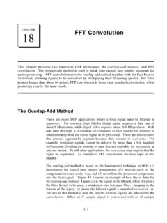
2 1*1211* 6* 4. 4*. 333* 2* 11* 6*6*. 3. 1. 1111*6* 6*. 66666. 6* 666 4444. 4 44444. 4 10. 10*. 10. 10. 10. 6*6 10. 10. 4 44 10. 1010. 10*. 10*. 1 x1. CSCE 666 Pattern Analysis | Ricardo Gutierrez-Osuna | CSE@TAMU 2. The histogram The simplest form of non-parametric DE is the histogram Divide the sample space into a number of bins and approximate the density at the center of each bin by the fraction of points in the training data that fall into the corresponding bin 1 # ( . =.. The histogram requires two parameters to be defined: bin width and starting position of the first bin 0 .1 6. 0 .1 4. 0 .1 2. 0 .1. p (x ) 0 .0 8. 0 .0 6. 0 .0 4. 0 .0 2. 0. 0 2 4 6 8 10 12 14 16 x CSCE 666 Pattern Analysis | Ricardo Gutierrez-Osuna | CSE@TAMU 3. The histogram is a very simple form of density estimation , but has several drawbacks The density estimate depends on the starting position of the bins For multivariate data, the density estimate is also affected by the orientation of the bins The discontinuities of the estimate are not due to the underlying density .)

3 They are only an artifact of the chosen bin locations These discontinuities make it very difficult (to the na ve analyst) to grasp the structure of the data A much more serious problem is the curse of dimensionality, since the number of bins grows exponentially with the number of dimensions In high dimensions we would require a very large number of examples or else most of the bins would be empty These issues make the histogram unsuitable for most practical applications except for quick visualizations in one or two dimensions Therefore, we will not spend more time looking at the histogram CSCE 666 Pattern Analysis | Ricardo Gutierrez-Osuna | CSE@TAMU 4. Non-parametric DE, general formulation Let us return to the basic definition of probability to get a solid idea of what we are trying to accomplish The probability that a vector , drawn from a distribution ( ), will fall in a given region of the sample space is = .. Suppose now that vectors (1 , (2 , ( are drawn from the distribution; the probability that of these vectors fall in is given by the binomial distribution.)))

4 = 1 .. It can be shown (from the properties of the binomial ) that the mean and variance of the ratio / are 2 1 . = and = = . N . Therefore, as the distribution becomes sharper (the variance gets smaller), so we can expect that a good estimate of the probability can be obtained from the mean fraction of the points that fall within .. [Bishop, 1995]. CSCE 666 Pattern Analysis | Ricardo Gutierrez-Osuna | CSE@TAMU 5. On the other hand, if we assume that is so small that ( ) does not vary appreciably within it, then .. where is the volume enclosed by region . Merging with the previous result we obtain . = .. This estimate becomes more accurate as we increase the number of sample points and shrink the volume . In practice the total number of examples is fixed To improve the accuracy of the estimate ( ) we could let approach zero but then would become so small that it would enclose no examples This means that, in practice, we will have to find a compromise for.

5 Large enough to include enough examples within . Small enough to support the assumption that ( ) is constant within . CSCE 666 Pattern Analysis | Ricardo Gutierrez-Osuna | CSE@TAMU 6. In conclusion, the general expression for non-parametric density estimation becomes .. where # .. # . When applying this result to practical density estimation problems, two basic approaches can be adopted We can fix and determine from the data. This leads to Kernel density estimation (KDE), the subject of this lecture We can fix and determine from the data. This gives rise to the k- nearest-neighbor (kNN) approach, which we cover in the next lecture It can be shown that both kNN and KDE converge to the true probability density as , provided that shrinks with , and that grows with appropriately CSCE 666 Pattern Analysis | Ricardo Gutierrez-Osuna | CSE@TAMU 7. Parzen windows Problem formulation Assume that the region that encloses the examples is a hypercube with sides of length centered at x h Then its volume is given by = , where is the number of dimensions h h To find the number of examples that fall within this region we define a Kernel function ( ).

6 1 < 1 2 = 1.. =. 0 . This Kernel , which corresponds to a unit hypercube centered at the origin, is known as a Parzen window or the na ve estimator The quantity (( ( )/ ) is then equal to unity if ( is inside a hypercube of side centered on , and zero otherwise [Bishop, 1995]. CSCE 666 Pattern Analysis | Ricardo Gutierrez-Osuna | CSE@TAMU 8. The total number of points inside the x hypercube is then 1 / V.. ( x (4 x (3 x (2 x (1 . = =1 .. V o lu m e Substituting back into the expression for the density estimate K ( x - x (1 ) = 1. x (1. 1 ( . = . =1 K ( x - x (2 ) = 1. x (2.. K ( x - x (3 ) = 1. Notice how the Parzen window x (3. estimate resembles the histogram, with the exception that the bin K ( x - x (4 ) = 0. locations are determined by the data x (4. CSCE 666 Pattern Analysis | Ricardo Gutierrez-Osuna | CSE@TAMU 9. To understand the role of the Kernel function we compute the expectation of the estimate . 1 ( . = =1.)))))))))))))))))

7 1 ( 1 ( . = = .. where we have assumed that vectors ( are drawn independently from the true density ( ). We can see that the expectation of is a convolution of the true density ( ) with the Kernel function Thus, the Kernel width plays the role of a smoothing parameter: the wider is, the smoother the estimate . For 0, the Kernel approaches a Dirac delta function and . approaches the true density However, in practice we have a finite number of points, so cannot be made arbitrarily small, since the density estimate would then degenerate to a set of impulses located at the training data points CSCE 666 Pattern Analysis | Ricardo Gutierrez-Osuna | CSE@TAMU 10. Exercise Given dataset = 4, 5, 5, 6, 12, 14, 15, 15, 16, 17 , use Parzen windows to estimate the density ( ) at = 3,10,15; use = 4. Solution Let's first draw the dataset to get an idea of the data y=15. p(x). y=3 y=10. 5 10 15 x Let's now estimate ( = 3). 1 ( 1 3 4 3 5 3 17.))))

8 =3 =.. =1 .. =. 10 41.. 4. + . 4. + . 4. = Similarly 1. = 10 = 0+0+0+0+0+0+0+0+0+0 =0. 10 4 1. 1. = 15 = 0 + 0 + 0 + 0 + 0 + 1 + 1 + 1 + 1 + 0 = 10 4 1. CSCE 666 Pattern Analysis | Ricardo Gutierrez-Osuna | CSE@TAMU 11. Smooth kernels The Parzen window has several drawbacks It yields density estimates that have discontinuities It weights equally all points , regardless of their distance to the estimation point . For these reasons, the Parzen window is commonly replaced with a smooth Kernel function ( ).. = 1. Usually, but not always, ( ) will be a radially symmetric and 1. /2 2 . unimodal pdf, such as the Gaussian = 2 . Which leads to the density estimate 1 ( . = . =1 . P arze n (u ) K (u ). 1. A=1 A=1. -1 /2 -1 /2 u -1 /2 -1 /2 u CSCE 666 Pattern Analysis | Ricardo Gutierrez-Osuna | CSE@TAMU 12. Interpretation Just as the Parzen window estimate can be seen as a sum of boxes centered at the data, the smooth Kernel estimate is a sum of bumps.)

9 The Kernel function determines the shape of the bumps The parameter , also called the smoothing parameter or bandwidth, determines their width 0 .0 4 5. D e n s it y 0 .0 4 e s tim a te 0 .0 3 5. 0 .0 3. P KD E (x); h = 3. 0 .0 2 5. K e rn e l f u n c tio n s 0 .0 2. 0 .0 1 5. 0 .0 1. 0 .0 0 5. 0. -1 0 -5 0 5 10 15 20 25 30 35 40. x D a ta CSCE 666 Pattern Analysis | Ricardo Gutierrez-Osuna | CSE@TAMU p o in ts 13. Bandwidth selection The problem of choosing is crucial in density estimation A large will over-smooth the DE and mask the structure of the data A small will yield a DE that is spiky and very hard to interpret P K DE(x); h= P K DE(x); h= 0 0. -10 -5 0 5 10 15 20 25 30 35 40 -10 -5 0 5 10 15 20 25 30 35 40. x x P K DE(x); h= P K DE(x); h= 0 0. -10 -5 0 5 10 15 20 25 30 35 40 -10 -5 0 5 10 15 20 25 30 35 40. x x CSCE 666 Pattern Analysis | Ricardo Gutierrez-Osuna | CSE@TAMU 14. We would like to find a value of that minimizes the error between the estimated density and the true density A natural measure is the MSE at the estimation point , defined by 2 2.

10 = + .. This expression is an example of the bias-variance tradeoff that we saw in an earlier lecture: the bias can be reduced at the expense of the variance, and vice versa The bias of an estimate is the systematic error incurred in the estimation The variance of an estimate is the random error incurred in the estimation CSCE 666 Pattern Analysis | Ricardo Gutierrez-Osuna | CSE@TAMU 15. The bias-variance dilemma applied to bandwidth selection simply means that A large bandwidth will reduce the differences among the estimates of for different data sets (the variance), but it will increase the bias of with respect to the true density ( ). A small bandwidth will reduce the bias of , at the expense of a larger variance in the estimates . BIAS VARIANCE. True density h= Multiple Kernel h= (x); h= density estimates P P (x);(x);. KDE. KDE. KDE. P. 0. 0-3 -2 -1 0 1 2 3 0. -3 -2 -1 x0 1 2 3 -3 -2 -1 0 1 2 3. x x CSCE 666 Pattern Analysis | Ricardo Gutierrez-Osuna | CSE@TAMU 16.