Transcription of Lab 2: Basic Concepts in Control System Design
1 ME C134 / EE C128 Fall 2017 Lab 2UC BerkeleyLab 2: Basic Concepts in Control System Design There is nothing worse than a sharp image of a fuzzy concept. Ansel Adams1 ObjectivesThe goal of this lab is to understand some of the Basic Concepts behind Control theory: equilibrium points,stability, feedback, steady-state response, and Poles and ZerosRecall that thepolesof a transfer function (TF) are those values of the Laplace transform variable,s, forwhich the denominator of the TF is zero, including any roots shared with the numerator, roots of thedenominator which cancel out with the numerator. Similarly, thezerosof a transfer function (TF) arethose values ofsthat cause the TF to become zero, including roots shared with the StabilityThe time response of a linear time invariant (LTI) dynamical systemc(t) =cforced(t) +cnatural(t), wherecforced(t) is the forced response (driven by the input applied to the System ) andcnatural(t) is the naturalresponse (driven by the System s initial states).
2 A linear, time-invariant System is called: stableif the natural response approaches zero as time approaches infinity. unstableif the natural response grows without bound as time approaches infinity. marginally stableif the natural response neither decays nor grows but remains constant or oscillatesas time approaches LTI dynamical systems one can discuss stability easily in terms of the locations of the poles of thesystem s TF. A System is stable if all poles lie in the left half of the complex plane (LHP). A systemis unstable if its TF has at least one pole in the right half of the complex plane (RHP), or a pole ofmultiplicity greater than one on the imaginary axis. A System is marginally stable if it has no poles inthe RHP and only poles of multiplicity one on the imaginary 14, 20171 of 4ME C134 / EE C128 Fall 2017 Lab 2UC Berkeley3 Simple feedback systemConsider the feedback System shown in Figure (s)Y(s)Figure 1: Simple proportional Control systemSuppose the Control goal is to track a step What are the poles and zeros of the open-loop System ?
3 Is the open-loop System stable? Can theopen-loop System track a step input? Suppose you use proportional feedback Control as shown in Figure 1. Explainwhythe scheme aboveis called proportional feedback. Explain (mathematically) how this scheme can be used to stabilizethe Is the System stable for all values ofK >0? Prove or find a For what values ofK >0 is the System completely oscillatory?5. For what values ofK >0 is the System stable? Nonlinear damped pendulumThe dynamics of a real plant are often nonlinear in nature. There is a plethora of interesting math-ematical and physical differences between linear and nonlinear systems. In this part, you study themathematical differences between linear and nonlinear versions of the pendulum with respect to equilib-rium a damped pendulum as in Figure 2: A damped pendulumSeptember 14, 20172 of 4ME C134 / EE C128 Fall 2017 Lab 2UC BerkeleyThe nonlinear equation of motion for the pendulum in Figure 2 is given by: +cml +glsin =Tcml2(1)Here is the angle of the pendulum from the vertical (in rad),cis the velocity damping term (in s 1),mis the mass of the pendulum (in kg),lis the length (in m),gis the acceleration due to gravity (in ms 2)andTcis the force input (inN m).
4 For this problem assume thatg= ms 2,l= m,m= kg,andc= s What is the nonlinear term in the pendulum equation above?2. Very often, you remove the nonlinearity in the plant by linearizing the plant about an operatingpoint. In this case, we will do a Taylor series expansion around = 0 for the nonlinearity anddisregard the nonlinear terms in the expansion. What are the first three terms in the Taylor seriesexpansion of the nonlinearity? What is the linearized version of the simple pendulum equation?4 Simple Feedback System1. Create a Simulink model of the simple feedback System shown in Figure Verify the System is oscillatory for the value(s) ofKthat you found in the Pre-Lab. You can testsome select values ofKin this interval. Plot the step response of the System ( the input signalshould be a step input which steps from 0 to 1 at timet0= 0) for four different values Verify the System is stable for values ofKin the corresponding interval you found in the can test some select values in this interval.
5 Plot the step response of the System for four differentvalues ofKin this interval (on the same graph).Report the location of the poles of the closedloop System for each value of Suppose we want our output response to not significantly exceed the final value of our input (step)signal. We can set a bound on our response using the maximum percent overshoot (%OS) thepercent by which the maximum value of the response exceeds the stead state (final) value. In thiscase, let us specify that we want the %OS to be less or equal than 25% for allt simulation(not math), determine for what values ofK(find a range precision of forbounds is good enough) the %OS is less or equal than 25%? Also show graphically that your boundsonKare correct (needs to be evident on the plot). Report the location of the closed loop poles forthis value of How do the poles of the System change as K increases?
6 Notice that in designing a Control System , we first analyzed the stability of our open-loop plant. If ouropen-loop plant is unstable, we use feedback to stabilize the System . Then we pick the values for theparameters in our Control law so our Control objective (in this case, a constraint on the percent overshoot)is achieved. Of course, there will generally also be other constraints (transient response for example).Satisfying all the Design requirements is the goal of Control 14, 20173 of 4ME C134 / EE C128 Fall 2017 Lab 2UC Nonlinear Damped Pendulum1. Model the nonlinear damped pendulum in Simulink. Note that this isnota feedback Control System you are building a block diagram representation of a plant! Instead of using derivatives, generatethe necessary signals backwards by using integrators. Why might using numerical derivatives bebad? To simplify updating the model, define variables and use them as parameters in the Simulinkblocks ( instead of directly using the value of the pendulum lengthlin the block, define a variablelin Matlab and use it in the Simulink block).
7 Include a figure of the Simulink model in your Plot the response of this System to a single pulse having amplitude 10 and width are several ways to generate such a pulse; one easy way is to use a pulse generator withlarge period ( 100 s) and suitable pulse width ( when using a period of 100 s). When youplot the graph, show the response for 70 seconds of time. To what value is the pendulum angleconverging to?Hint:At some point you should also plot your pulse input to verify that it is thecorrect amplitude and width. This does not need to be included in your lab report, but will helpyou avoid Plot the response of this System to a pulse having amplitude 250 and width seconds. To whatnew value does the pendulum angle converge? Explain Replace the nonlinear term in your Simulink model with the linear version. Repeat the experimentfor the pulse with amplitude 10 and width seconds.
8 Do the nonlinear and linear versions agreefor the angle response?5. Now try the linear version with the pulse having amplitude 250 and width seconds. Do thenonlinear and linear versions agree for the angle response? Why is there a discrepancy?6. Based on your results from parts 4 and 5, when is the linearized System a good approximation ofthe original System ?September 14, 20174 of 4