Transcription of Lecture 1: Stochastic Volatility and Local Volatility - ku
1 Lecture 1: Stochastic Volatility andLocal VolatilityJim Gatheral, Merrill lynch Case Studies in Financial Modelling Course Notes,Courant Institute of Mathematical Sciences,Fall Term, 2002 AbstractIn the course of the following lectures, we will study why equityoptions are priced as they are. In so doing, we will apply many ofthe techniques students will have learned in previous semesters anddevelop some intuition for the pricing of both vanilla and exotic equityoptions. By considering specific examples, we will see that in pricingoptions, it is often as important to take into account the dynamics ofunderlying variables as it is to match known market prices of otherclaims. My hope is that these lectures will prove particularly usefulto those who end up specializing in the structuring, pricing, tradingand risk management of equity derivatives.
2 I am indebted to peter Friz for carefully reading these notes, providing correctionsand suggesting useful Stochastic MotivationThat it might make sense to model Volatility as a random variable should beclear to the most casual observer of equity markets. To be convinced, oneonly needs to remember the stock market crash of October 1987. Neverthe-less, given the success of the Black-Scholes model in parsimoniously describ-ing market options prices, it s not immediately obvious what the benefits ofmaking such a modelling choice might Volatility models are useful because they explain in a self-consistent way why it is that options with different strikes and expirationshave different Black-Scholes implied volatilities ( implied volatilities fromnow on) the Volatility smile.
3 In particular, traders who use the Black-Scholes model to hedge must continuously change the Volatility assumptionin order to match market prices. Their hedge ratios change accordingly inan uncontrolled way. More interestingly for us, the prices of exotic optionsgiven by models based on Black-Scholes assumptions can be wildly wrongand dealers in such options are motivated to find models which can take thevolatility smile into account when pricing Figure 1, we see that large moves follow large moves and smallmoves follow small moves (so called Volatility clustering ). From Figures 2and 3 (which shows details of the tails of the distribution), we see that thedistribution of stock price returns is highly peaked and fat-tailed relative tothe Normal distribution.
4 Fat tails and the high central peak are character-istics of mixtures of distributions with different variances. This motivatesus to model variance as a random variable. The Volatility clustering featureimplies that Volatility (or variance) is auto-correlated. In the model, this isa consequence of the mean reversion of is a simple economic argument which justifies the mean reversionof Volatility (the same argument that is used to justify the mean reversionof interest rates). Consider the distribution of the Volatility of IBM in onehundred years time say. If Volatility were not mean-reverting ( thedistribution of Volatility were not stable), the probability of the volatilityof IBM being between 1% and 100% would be rather low. Since we believethat it is overwhelmingly likely that the Volatility of IBM would in fact lie1 Note that simple jump-diffusion models do not have this property.
5 After a jump, thestock price Volatility does not 1: SPX daily log returns from 1/1/1990 to 31/12 2: Frequency distribution of SPX daily log returns from 1/1/1990 to31/12/1999 compared with the Normal that range, we deduce that Volatility must be motivated the description of variance as a mean-reverting randomvariable, we are now ready to derive the valuation 3: Tails of SPX frequency Derivation of the Valuation EquationIn this section, we follow Wilmott (1998) closely. We suppose that the stockpriceSand its variancevsatisfy the following SDEs:dS(t) = (t)S(t)dt+ v(t)S(t)dZ1(1)dv(t) = (S, v, t)dt+ (S, v, t) v(t)dZ2(2)with dZ1dZ2 = dtwhere (t) is the (deterministic) instantaneous drift of stock price returns, is the Volatility of Volatility and is the correlation between random stockprice returns and changes inv(t).
6 DZ1anddZ2are Wiener Stochastic process (1) followed by the stock price is equivalent to theone assumed in the derivation of Black and Scholes (1973). This ensures thatthe standard time-dependent Volatility version of the Black-Scholes formula(as derived in section of Wilmott (1998) for example) may be retrievedin the limit 0. In practical applications, this is a key requirement of astochastic Volatility option pricing model as practitioners intuition for thebehavior of option prices is invariably expressed within the framework of theBlack-Scholes the Black-Scholes case, there is only one source of randomness thestock price, which can be hedged with stock. In the present case, randomchanges in Volatility also need to be hedged in order to form a riskless port-folio.
7 So we set up a portfolio containing the option being priced whosevalue we denote byV(S, v, t), a quantity of the stock and a quantity 1of another asset whose valueV1depends on Volatility . We have =V S 1V1 The change in this portfolio in a timedtis given byd ={ V t+12v S2(t) 2V S2+ v S(t) 2V v S+12 2v 2 2V v2}dt 1{ V1 t+12v S2(t) 2V1 S2+ v S(t) 2V1 v S+12 2v 2 2V1 v2}dt+{ V S 1 V1 S }dS+{ V v 1 V1 v}dvTo make the portfolio instantaneously risk-free, we must choose V S 1 V1 S = 0to eliminatedSterms, and V v 1 V1 v= 0to eliminatedvterms. This leaves us withd ={ V t+12v S2 2V S2+ v S 2V v S+12 2v 2 2V v2}dt 1{ V1 t+12v S2 2V1 S2+ v S 2V1 v S+12 2v 2 2V1 v2}dt=r dt=r(V S 1V1)dtwhere we have used the fact that the return on a risk-free portfolio mustequal the risk-free raterwhich we will assume to be deterministic for our5purposes.
8 Collecting allVterms on the left-hand side and allV1terms onthe right-hand side, we get V t+12v S2 2V S2+ v S 2V v S+12 2v 2 2V v2+rS V S rV V v= V1 t+12v S2 2V1 S2+ v S 2V1 v S+12 2v 2 2V1 v2+rS V1 S rV1 V1 vThe left-hand side is a function ofVonly and the right-hand side is a functionofV1only. The only way that this can be is for both sides to be equal tosome functionfof theindependentvariablesS,vandt. We deduce that V t+12v S2 2V S2+ v S 2V v S+12 2v 2 2V v2+rS V S rV= ( ) V v(3)where, without loss of generality, we have written the arbitrary functionfofS,vandtas ( ). Conventionally, (S, v, t) is called the marketprice of Volatility risk because it tells us how much of the expected returnofVis explained by the risk ( deviation) ofvin the CapitalAsset Pricing Model Local HistoryGiven the computational complexity of Stochastic Volatility models and theextreme difficulty of fitting parameters to the current prices of vanilla op-tions, practitioners sought a simpler way of pricing exotic options consis-tently with the Volatility skew.
9 Since before Breeden and Litzenberger(1978), it was understood that the risk-neutralpdfcould be derived from themarket prices of European options. The breakthrough came when Dupire(1994) and Derman and Kani (1994) noted that under risk-neutrality, therewas a unique diffusion process consistent with these distributions. The cor-responding unique state-dependent diffusion coefficient L(S, t) consistentwith current European option prices is known as the Local Volatility is unlikely that Dupire, Derman and Kani ever thought of Local volatil-ity as representing a model of how volatilities actually evolve. Rather, it is6likely that they thought of Local volatilities as representing some kind ofaverage over all possible instantaneous volatilities in a Stochastic volatilityworld (an effective theory ).
10 Local Volatility models do not therefore reallyrepresent a separate class of models; the idea is more to make a simplify-ing assumption that allows practitioners to price exotic options consistentlywith the known prices of vanilla if any proof had been needed, Dumas, Fleming, and Whaley (1998)performed an empirical analysis which confirmed that the dynamics of theimplied Volatility surface were not consistent with the assumption of constantlocal section , we will show that Local Volatility is indeed an averageover instantaneous volatilities, formalizing the intuition of those practition-ers who first introduced the A Brief Review of Dupire s WorkFor a given expirationTand current stock priceS0, the collection{C(S0, K, T) ;K (0, )}of undiscounted option prices of different strikesyields the risk neutral density function of the final spotSTthrough therelationshipC(S0, K, T) = KdST (ST, T;S0) (ST K)Differentiate this twice with respect toKto obtain (K, T;S0) = 2C K2so the Arrow-Debreu prices for each expiration may be recovered by twicedifferentiating the undiscounted option price with respect toK.