Transcription of Lecture 11 Transmission Lines - Purdue University
1 Lecture 11 Transmission Transmission line TheoryFigure : Transmission Lines were the first electromagnetic waveguides ever invented. The were drivenby the needs in telegraphy technology. It is best to introduce Transmission line theory fromthe viewpoint of circuit theory. This theory is also discussed in many textbooks and lecture101102 Electromagnetic Field Theorynotes. Transmission Lines are so important in modern day electromagnetic engineering, thatmost engineering electromagnetics textbooks would be incomplete without introducing thetopic [29, 31, 38, 47, 48, 59, 71, 75, 77].Circuit theory is robust and is not sensitive to the detail shapes of the components in-volved such as capacitors or inductors.
2 Moreover, many Transmission line problems cannotbe analyzed with the full form of Maxwell s equations,1but approximate solutions can beobtained using circuit theory in the long-wavelength limit. We shall show that circuit theoryis an approximation of electromagnetic field theory when the wavelength is very long: thelonger the wavelength, the better is the approximation [47].Examples of Transmission Lines are shown in Figure The symbol for a transmissionline is usually represented by two pieces of parallel wires, but in practice, these wires neednot be : Courtesy of slides by A. Wadhwa, Dal, N. Malhotra [78].Circuit theory also explains why waveguides can be made sloppily when wavelength is longor the frequency low.
3 For instance, in the long-wavelength limit, we can make twisted-pairwaveguides with abandon, and they still work well (see Figure ). Hence, we shall firstexplain the propagation of electromagnetic signal on a Transmission line using circuit Time-Domain AnalysisWe will start with performing the time-domain analysis of a simple, infinitely long trans-mission line . Remember that two pieces of metal can accumulate attractive charges betweenthem, giving rise to capacitive coupling, electric field, and hence stored energy in the electricfield. Moreover, a piece of wire carrying a current generates a magnetic field, and hence,yielding stored energy in the magnetic field.
4 These stored energies are the sources of thecapacitive and inductive effects. But these capacitive and inductive effects are distributedover the spatial dimension of the Transmission line . Therefore, it is helpful to think of thetwo pieces of metal as consisting of small segments of metal concatenated together. Each ofthese segments will have a small inductance, as well as a small capacitive coupling betweenthem. Hence, we can model two pieces of metal with a distributed lumped element model asshown in Figure For simplicity, we assume the other conductor to be a ground plane,so that it need not be approximated with lumped called full-wave Lines103In the Transmission line , the voltageV(z,t) andI(z,t) are functions of both spacezandtimet, but we will model the space variation of the voltage and current with discrete stepapproximation.
5 The voltage varies from node to node while the current varies from branchto branch of the lump-element :First, we recall that the V-I relation of an inductor isV0=L0dI0dt( )whereL0is the inductor,V0is the time-varying voltage drop across the inductor, andI0isthe current through the inductor. Then using this relation between node 1 and node 2, wehaveV (V+ V) =L z I t( )The left-hand side is the voltage drop across the inductor, while the right-hand side followsfrom the aforementioned V-I relation of an inductor, but we have replacedL0=L z. Here,Lis the inductance per unit length ( line inductance) of the Transmission line . AndL zisthe incremental inductance due to the small segment of metal of length z.
6 Then the abovecan be simplified to V= L z I t( )Next, we make use of the V-I relation for a capacitor, which isI0=C0dV0dt( )whereC0is the capacitor,I0is the current through the capacitor, andV0is a time-varyingvoltage drop across the capacitor. Thus, applying this relation at node 2 gives I=C z t(V+ V) C z V t( )104 Electromagnetic Field TheorywhereCis the capacitance per unit length, andC zis the incremental capacitance betweenthe small piece of metal and the ground plane. In the above, we have used Kirchhoff currentlaw to surmise that the current through the capacitor is I, where I=I(z+ z,t) I(z,t).In the last approximation in ( ), we have dropped a term involving the product of zand V, since it will be very small or second order in the limit when z 0, one gets from ( ) and ( ) that V(z,t) z= L I(z,t) t( ) I(z,t) z= C V(z,t) t( )The above are the telegrapher s equations.
7 They are two coupled first-order equations, andcan be converted into second-order equations easily. Therefore, 2V z2 LC 2V t2= 0( ) 2I z2 LC 2I t2= 0( )The above are wave equations that we have previously studied, where the velocity of the waveis given byv=1 LC( )Furthermore, if we assume thatV(z,t) =f+(z vt)( )a right-traveling wave, and substituting it into ( ) yields L I t=f +(z vt)( )SubstitutingV(z,t) into ( ) yields I z=Cvf +(z vt)( )The above implies thatI= CLf+(z vt)( )Consequently,V(z,t)I(z,t)= LC=Z0( ) Transmission Lines105whereZ0is the characteristic impedance of the Transmission line . The above ratio is onlytrue for one-way traveling wave, in this case, one that propagates in the + a wave that travels in the negativezdirection, ,V(z,t) =f (z+vt)( )with the correspondingI(z,t) derived, one can show thatV(z,t)I(z,t)= LC= Z0( )Time-domain analysis is very useful for transient analysis of Transmission Lines , especiallywhen nonlinear elements are coupled to the Transmission line .
8 Another major strength oftransmission line model is that it is a simple way to introduce time-delay in a circuit. Timedelay is a wave propagation effect, and it is harder to incorporate into circuit theory or apure circuit model consisting ofR,L, andC. In circuit theory, Laplace s equation is usuallysolved, which is equivalent to Helmholtz equation with infinite wave velocity, namely,limc 2 (r) + 2c2 (r) = 0= 2 (r) = 0( )Hence, events in Laplace s equation happen Frequency-Domain AnalysisFrequency domain analysis is very popular as it makes the Transmission line equations verysimple. Moreover, generalization to a lossy system is quite straight forward.
9 Furthermore, forlinear time invariant systems, the time-domain signals can be obtained from the frequency-domain data by performing a Fourier inverse a time-harmonic signal on a Transmission line , one can analyze the problem in thefrequency domain using phasor technique. A phasor variable is linearly proportional to aFourier transform variable. The telegrapher s equations ( ) and ( ) then becomeddzV(z, ) = j LI(z, )( )ddzI(z, ) = j CV(z, )( )The corresponding Helmholtz equations are thend2 Vdz2+ 2 LCV= 0( )d2 Idz2+ 2 LCI= 0( )The general solutions to the above areV(z) =V+e j z+V ej z( )I(z) =I+e j z+I ej z( )106 Electromagnetic Field Theorywhere = LC.
10 This is similar to what we have seen previously for plane waves in theone-dimensional wave equation in free space, whereEx(z) =E0+e jk0z+E0 ejk0z( )wherek0= 0 0. We see a much similarity between ( ), ( ), and ( ).To see the solution in the time domain, we letV =|V |ej , and the voltage signalabove can be converted back to the time domain asV(z,t) =<e{V(z, )ej t}( )=|V+|cos( t z+ +) +|V |cos( t+ z+ )( )As can be seen, the first term corresponds to a right-traveling wave, while the second term isa left-traveling , if we assume only a one-way traveling wave to the right by lettingV =I = 0, then it can be shown that, for a right-traveling waveV(z)I(z)=V+I+= LC=Z0( )In the above, the telegrapher s equations, ( ) or ( ) have been used to find arelationship betweenI+andV+.