Lecture 13 - Heat Transfer Applied Computational Fluid ...

1 Lecture 13 - heat Transfer Applied Computational Fluid Dynamics Instructor: Andr Bakker Andr Bakker (2002-2006). Fluent Inc. (2002). 1. Introduction Typical design problems involve the determination of: Overall heat Transfer coefficient, for a car radiator. Highest (or lowest) temperature in a system, in a gas turbine, chemical reaction vessels, food ovens. Temperature distribution (related to thermal stress), in the walls of a spacecraft. Temperature response in time dependent heating/cooling problems, engine cooling, or how fast does a car heat up in the sun and how is it affected by the shape of the windshield? 2. Modes of heat Transfer Conduction: diffusion of heat due to temperature gradients. A. measure of the amount of conduction for a given gradient is the heat conductivity.

2 Convection: when heat is carried away by moving Fluid . The flow can either be caused by external influences, forced convection; or by buoyancy forces, natural convection. Convective heat Transfer is tightly coupled to the Fluid flow solution. Radiation: Transfer of energy by electromagnetic waves between surfaces with different temperatures, separated by a medium that is at least partially transparent to the (infrared) radiation. Radiation is especially important at high temperatures, during combustion processes, but can also have a measurable effect at room temperatures. 3. Overview dimensionless numbers Nusselt number: Nu = hL / k f . Ratio between total heat Transfer in a convection dominated system and the estimated conductive heat Transfer .

3 Grashof number: Gr = L3 g / 2 w . Ratio between buoyancy forces and viscous forces. Prandtl number: Pr = c p / k . Ratio between momentum diffusivity and thermal diffusivity. Typical values are Pr = for liquid metals; Pr = for most gases; Pr = 6 for water at room temperature. Rayleigh number: Ra = Gr Pr = L3 2 g c p T / k = L3 g T / . The Rayleigh number governs natural convection phenomena. Reynolds number: Re = UL / . Ratio between inertial and viscous forces. 4. Enthalpy equation In CFD it is common to solve the enthalpy equation, subject to a wide range of thermal boundary conditions. Energy sources due to chemical reaction are included for reacting flows. Energy sources due to species diffusion are included for multiple species flows.

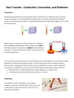
4 The energy source due to viscous heating describes thermal energy created by viscous shear in the is important when the shear stress in the Fluid is large ( lubrication) and/or in high-velocity, compressible flows. Often, however, it is negligible. In solid regions, a simple conduction equation is usually solved, although convective terms can also be included for moving solids. 5. Conjugate heat Transfer Conjugate heat Transfer refers to the ability to compute conduction of heat through solids, coupled with convective Grid heat Transfer in a Fluid . Coupled boundary conditions are available for wall zones that Velocity vectors separate two cell zones. Either the solid zone or the Fluid zone, or both, may contain heat sources. Temperature contours The example here shows the temperature profile for coolant Example: Cooling flow over fuel rods flowing over fuel rods that generate heat .

5 6. Periodic heat Transfer Also known as streamwise-periodic or fully-developed flow. Used when flow and heat Transfer patterns are repeated, : Compact heat exchangers. Flow across tube banks. Geometry and boundary conditions repeat in streamwise direction. inflow outflow Outflow at one periodic boundary is inflow at the other 7. heat conduction - Fourier's law The heat flux is proportional to the temperature gradient: Q. = q = k T. A. where k(x,y,z,T) is the thermal temperature conductivity. profile In most practical situations dT. conduction, convection, and dx hot wall cold wall radiation appear in combination. Also for convection, the heat Transfer coefficient is important, x because a flow can only carry heat away from a wall when that wall is conducting.

6 8. Generalized heat diffusion equation If we perform a heat balance on a small volume of material . heat conduction T heat conduction in q& out heat generation we get: T. c = k 2T + q&. t rate of change heat cond. heat of temperature in/out generation k = = thermal diffusivity c 9. Conduction example Compute the heat Transfer through the wall of a home: Tout = 20 F Tout = 68 F. Although slight, you can see the thermal bridging effect through the studs 2x6 stud k= W/m2-K. sheetrock shingles k= W/m2-K. k= W/m2-K fiberglass sheathing insulation 2. k= W/m -K k= W/m2-K. 10. Convection heat Transfer Convection is movement of heat with a Fluid . , when cold air sweeps past a warm body, it draws away warm air near the body and replaces it with cold air.

7 Flow over a heated block 11. Forced convection example Developing flow in a pipe (constant wall temperature). Tw T . T Tw T Tw T Tw T. Tw bulk Fluid temperature heat flux from wall x 12. Thermal boundary layer Just as there is a viscous boundary layer in the velocity distribution, there is also a thermal boundary layer. Thermal boundary layer thickness is different from the thickness of the (momentum) viscous sublayer, and Fluid dependent. The thickness of the thermal sublayer for a high-Prandtl-number Fluid ( water) is much less than the momentum sublayer thickness. For fluids of low Prandtl numbers ( liquid metal), it is much larger than the momentum sublayer thickness. thermal boundary velocity boundary layer edge layer edge T . y T , U.

8 T t L. T ( y) . Tw Tw 13. Natural convection Natural convection (from a heated vertical plate). T = (T ). As the Fluid is warmed by the Tw plate, its density decreases and a buoyant force arises which induces flow in the vertical direction. The force is u proportional to ( ) g . The dimensionless group that governs natural convection is the Rayleigh number: gravity T , . g TL3. Ra = =.. Typically: Nu Ra x 1. 4. < x < 13. 14. Natural convection around a person Light weight warm air tends to move upward when surrounded by cooler air. Thus, warm-blooded animals are surrounded by thermal plumes of rising warm air. This plume is made visible by means of a Schlieren optical system that is based on the fact that the refraction of light through a gas is dependent on the density of the gas.

9 Although the velocity of the rising air is relatively small, the Reynolds number for this flow is on the order of 3000. 15. Natural convection - Boussinesq model Makes simplifying assumption that density is uniform. Except for the body force term in the momentum equation, which is replaced by: ( 0 ) g = 0 ( T T0 ) g Valid when density variations are small ( small variations in T). Provides faster convergence for many natural-convection flows than by using Fluid density as function of temperature because the constant density assumptions reduces non-linearity. Natural convection problems inside closed domains: For steady-state solver, Boussinesq model must be used. Constant density o allows mass in volume to be defined. For unsteady solver, Boussinesq model or ideal gas law can be used.

10 Initial conditions define mass in volume. 16. Newton's law of cooling Newton described the cooling of objects with an arbitrary shape in a pragmatic way. He postulated that the heat Transfer Q is proportional to the surface area A of the object and a temperature difference T. The proportionality constant is the heat Transfer coefficient h(W/m2-K). This empirical constant lumps together all the information about the heat Transfer process that we don't know or don't understand. T . q Tbody Q = q A = h A (Tbody T ) = h A T. h= average heat Transfer coefficient (W/m2-K) 17. heat Transfer coefficient h is not a constant, but h = h( T). Three types of convection. Natural convection. Fluid moves Typical values of h: due to buoyancy. Thot Tcold 4 - 4,000 W/m2-K.