Transcription of Lecture 9: Hidden Markov Models
1 Lecture 9: Hidden Markov Models Working with time series data Hidden Markov Models Inference and learning problems Forward-backward algorithm Baum-Welch algorithm for parameter fittingCOMP-652 and ECSE-608, Lecture 9 - February 9, 20161 Time series/sequence data Very important in practice: Speech recognition Text processing (taking into account the sequence of words) DNA analysis Heart-rate monitoring Financial market forecasting Mobile robot sensor processing .. Does this fit the machine learning paradigm as described so far? The sequences arenot all the same length(so we cannot just assumeone attribute per time step) The data at each time slice/index isnot independent The data distributionmay change over timeCOMP-652 and ECSE-608, Lecture 9 - February 9, 20162 Example: Robot position tracking1 Illustrative Example: Robot Localization!
2 "Probt=0 Sensory model: never more than 1 mistakeMotion model: may not execute action with small Pfeiffer, 2004 COMP-652 and ECSE-608, Lecture 9 - February 9, 20163 Example (II)Illustrative Example: Robot Localization!"Probt=1 COMP-652 and ECSE-608, Lecture 9 - February 9, 20164 Example (III)Illustrative Example: Robot Localization!"Probt=3 COMP-652 and ECSE-608, Lecture 9 - February 9, 20165 Example (IV)Illustrative Example: Robot Localization!"Probt=4 COMP-652 and ECSE-608, Lecture 9 - February 9, 20166 Example (V)Illustrative Example: Robot Localization!"#$Trajectory!%Probt=5 COMP-652 and ECSE-608, Lecture 9 - February 9, 20167 Hidden Markov Models (HMMs) Hidden Markov Models (HMMs) are used for situations in which: The data consists of asequence of observations The observations depend (probabilistically) on the internal state of adynamical system The true state of the system is unknown( , it is a Hidden or latentvariable) There are numerous applications, including: Speech recognition Robot localization Gene finding User modelling Fetal heart rate monitoring.
3 COMP-652 and ECSE-608, Lecture 9 - February 9, 20168 How an HMM works Assume a discrete clockt= 0,1,2,.. At eacht, the system is in some internal ( Hidden ) stateSt=sand anobservationOt=ois emitted (stochastically)based only ons(Random variables are denoted with capital letters) The system transitions (stochastically) to a new stateSt+1, accordingto a probability distributionP(St+1|St), and the process repeats. This interaction can be represented as a graphical model (recall thateach circle is a random variable,StorOtin this case):s1s2s3s4o1o2o3o4 Markov assumption:St+1 St 1|St(future is independent of the pastgiven the present)COMP-652 and ECSE-608, Lecture 9 - February 9, 20169 HMM definitions1s2s3s4o1o2o3o4 An HMM consists of: Aset of statesS(usually assumed to be finite) Astart state distributionP(S1=s), s SThis annotates the top left node in the graphical model State transition probabilities.
4 P(St+1=s |St=s), s,s SThese annotate the right-going arcs in the graphical model Aset of observationsO(often assumed to be finite) Observation emission probabilitiesP(Ot=o|St=s), s S,o annotate the down-going arcs above The model ishomogeneous: the transition and emission probabilitiesdonot depend on time, only on the states/observationsCOMP-652 and ECSE-608, Lecture 9 - February 9, 201610 Finite HMMs IfSandOare finite, the initial state distribution can be represented asa vectorb0of size|S| Transition probabilities form a matrixTof size|S| |S|; each rowiisthe multinomial of the next state given that the current state isi Similarly, the emission probabilities form a matrixQof size|S| |O|;each row is a multinomial distribution over the observations, given thestate.
5 Together,b0,TandQform themodelof the HMM. IfOis not not finite, the multinomial can be replaced with an appropriateparametric distribution ( Normal) IfSis not finite, the model is usually not called an HMM, and differentways of expressing the distributions may be used, Kalman filter Extended Kalman filter ..COMP-652 and ECSE-608, Lecture 9 - February 9, 201611 Examples Gene regulation O={A,C,G,T} S={Gene,Transcription factor binding site,Junk DNA,..} Speech processing O=speech signal S=word or phoneme being uttered Text understanding O=words S=topic ( sports, weather, etc) Robot localization O=sensor readings S=discretized position of the robotCOMP-652 and ECSE-608, Lecture 9 - February 9, 201612 HMM problems How likely is a given observation sequence,o0,o1.
6 OT? , computeP(O1=o1,O2=o2,..OT=oT) Given an observation sequence, what is the probability distribution forthe current state? , computeP(ST=s|O1=o1,O2=o2,..OT=oT) What is the most likely state sequence for explaining a given observationsequence? ( Decoding problem )arg maxs1,..sTP(S1=s1,..ST=sT|O1=o1,..OT=oT) Given one (or more) observation sequence(s), compute the modelparametersCOMP-652 and ECSE-608, Lecture 9 - February 9, 201613 Computing the probability of an observation sequence Very useful in learning for: Seeing if an observation sequence is likely to be generated by acertain HMM from a set of candidates (often used in classification ofsequences) Evaluating if learning the model parameters is working How to do it:belief propagationCOMP-652 and ECSE-608, Lecture 9 - February 9, 201614 Decomposing the probability of an observation sequences1s2s3s4o1o2o3o4P(o1.)
7 OT) = s1,..sTP(o1,..oT,s1,..sT)= s1,..sTP(s1)(T t=2P(st|st 1))(T t=1P(ot|st))(using the model)= sTP(oT|sT) s1,..sT 1P(sT|sT 1)P(s1)(T 1 t=2P(st|st 1))(T 1 t=1P(ot|st))This form suggests a dynamic programming solution!COMP-652 and ECSE-608, Lecture 9 - February 9, 201615 Dynamic programming idea By inspection of the previous formula, note that we actually wrote:P(o1,o2,..oT) = sTP(o1,o2,..oT,sT)= sTP(oT|sT) sT 1P(sT|sT 1)P(o1,..oT 1,sT 1) The variables for the dynamic programming will beP(o1,o2,..ot,st).COMP-652 and ECSE-608, Lecture 9 - February 9, 201616 The forward algorithm Given an HMM model and an observation sequenceo1,..oT, define: t(s) =P(o1,..ot,St=s) We can put these variables together in a vector tof sizeS.
8 In particular, 1(s) =P(o1,S1=s) =P(o1|S1=s)P(S1=s) =qso1b0(s) Fort= 2,..T, t(s) =psot s ps s t 1(s ) The solution is thenP(o1,..oT) = s T(s)COMP-652 and ECSE-608, Lecture 9 - February 9, 201617 Example12345 Consider the 5-state hallway shown above The start state is always state 3 The observation is the number of walls surrounding the state (2 or 3) There is of staying in the same state, moving left or right; if the movement would lead to a wall, the stateis statesee and ECSE-608, Lecture 9 - February 9, 201618 Example: Forward algorithm12345 Timet1 Obs2 t(1) t(2) t(3) t(4) t(5) and ECSE-608, Lecture 9 - February 9, 201619 Example: Forward algorithm12345 Timet12 Obs22 t(1) t(2) t(3) t(4) t(5) and ECSE-608, Lecture 9 - February 9, 201620 Example: Forward algorithm: two different observationsequences12345 Timet123 Obs222 t(1) t(2) t(3) t(4) t(5) t(1) t(2) t(3) t(4) t(5) and ECSE-608, Lecture 9 - February 9, 201621 Example.
9 Forward algorithm12345 Timet12345678910 Obs2232322233 t(1) t(2) t(3) t(4) t(5) Note that probabilities decrease with the length of the sequence This is due to the fact that we are looking at a joint probability; thisphenomenon would not happen for conditional probabilities This can be a source of numerical problems for very long and ECSE-608, Lecture 9 - February 9, 201622 Conditional probability queries in an HMM Because the state is never observed, we are often interested toinfer itsconditional distributionfrom the observations. There are several interesting types of queries: Monitoring (filtering, belief state maintenance): what is the currentstate, given the past observations?
10 Prediction: what will the state be in several time steps, given the pastobservations? Smoothing (hindsight): update the state distribution of past timesteps, given new data Most likely explanation: compute the most likely sequence of statesthat could have caused the observation sequenceCOMP-652 and ECSE-608, Lecture 9 - February 9, 201623 Belief state monitoring Given an observation sequenceo1,..ot, thebelief stateof an HMM attime steptis defined as:bt(s) =P(St=s|o1,..ot)Note that ifSis finitebtis a probability vector of sizeS(so its elementssum to1) In particular,b1(s) =P(S1=s|o1) =P(S1=s,o1)P(o1)=P(S1=s,o1) s P(S1=s ,o1)=b0(s)qso1 s b0(s )qs o1 To compute this, we would assign:b1(s) b0(s)qso1and then normalize it (dividing by sb1(s))COMP-652 and ECSE-608, Lecture 9 - February 9, 201624 Updating the belief state after a new observations1s2s3s4o1o2o3o4 Suppose we havebt(s)and we receive a new observationot+1.