Transcription of Lecture n2 Turbulent flow Modelling - Politechnika …
1 Turbulent flowHenryk KudelaContents1 Turbulence modeling12 Velocity profiles: the inner, outer, and overlap Solution .. velocity profile ..83 Turbulence: some important thoughts124 Problems141 Turbulence modelingWe will be assume constant density and viscosity of fluid. We also assume that no thermal inter-action of the fluid with the solid boundary. In this way only continuity and momentum equationsdescribe fluid velocity(u,v,w)and pressurepdistribution (Navier -Stokes equation): v t+v v= 1 p+ vmomentum equation(1) v= u x+ v y+ w z=0continuity equation conservation of mass(2)Equations (1),(2) are subjected to no slip boundary condition at the walls and knows inlet and laminar and Turbulent flows satisfy (1),(2). For laminar flow, where there are no randomfluctuations, we can sometimes solve them for a variety of geometries, like flow in pipe (see lec-ture n5 viscous flow).
2 Most flows encountered in engineering practice are Turbulent . This isparticularly true for pipe flows , so it is essential at this time to introduce a few very fundamentalnotions that will lead us to a better physical understandingof the friction factors, and hence thepressure losses, in such flows . It is useful to begin by recalling the difference in the nature of ve-locity profiles between laminar and Turbulent flow in duct. This is depicted in The parabolicprofile of part (a) corresponds to a fully-developed Poiseuille flow for which it can be seen that1 Figure 1: Comparison of laminar and Turbulent velocity profiles in duct; a) laminar , b) turbulentthe velocity gradient at the wall, and hence also the wall shear stress, w, is not so large as in theturbulent case of part (b) representing the (time) mean flow for fully-developed turbulence.
3 Theregion very close to the wall exhibits a nearly linear velocity profile in the Turbulent case, andis completely dominated by viscous effects. This inner layer is termed as theviscous sublayer;velocity varies linearly with distance from the wall. The so-called outer region or called alsoasinertial sublayer, shows nearly constant velocity with distance from the wall. But we recognizethat this outer layer velocity cannot satisfy the no slip condition at the wall, and at the same timethe inner (linear) profile whichdoessatisfy no slip condition (u=0) will not correctly asymptoteto the outer solution. This suggests that a third solution, overlap layer ,is needed to match thesetwo thickness of the viscous sublayer is very small (typically, much less than 1 percent of the pipediameter), but this thin layer next to the wall plays a dominant role on characteristics because oflarge velocity gradients it Turbulent flow, because of the fluctuations, every velocity and pressure term in (1),(2) is arapidly varying random function of time and 2: Graphical depiction of components of Reynolds decomposition2At present our mathematics cannot handle such instantaneous fluctuating variables.
4 No singlepair of random functionsu(x,y,z,t)andp(x,y,z,t)is known to be a solution to (1),(2). As engi-neers we are interested more in the average, mean values of velocity, pressure, shear stress, approach led Osborne Reynolds in 1895 to the decomposition, now known as the Reynoldsdecompositionu(x,y,z,t) =u+u (x,y,z,t),v(x,y,z,t) =v+v ,w(x,y,z,t) =w+w ,p(x,y,z,t) =p+p (3)In equation (3) the bar ( ) denotes a time average,and prime ( ) indicates fluctuation aboutthe time averaged, mean quantity. Formally, time average is defined byu=limT 1T T0udt(4)The fluctuationu is defined as the deviation of u from its average valueu =u uand bydefinition a fluctuation has zero mean =limT 1T T0(u u)dt=u u=0(5)For a time average to make sense, the integrals (4) and (??) have to be independent form initialtimet=0. It means that the mean flow has to be statistically steady: u t=0.
5 (6)The mean square of a fluctuation is not zerou 2>0 and is a measure of theintensity of theturbulence:u 2=limT 1T T0u 2dt6=0(7)Also in general the mean fluctuation products such asu v ,u p is not equal zero in a typicalturbulent flow. Substitute (3) into Navier Stokes equations (1),(2), and take the time mean ofeach equation. The continuity relation reduces to u x+ v y+ w z=0(8)which is no different from a laminar continuity relation (2). We can aslso show easily that u x+ v y+ w z=0.(9)So (8) and (9) tell us that the mean and fluctuating parts of velocity field each satisfy the interesting is what happens to the equation for the momentum (1). Let us write the the firstu component of this equation: u t+u u x+v u y+w u z= 1 p x+ ( 2u x2+ 2u y2+ 2u z2)(10)3 The left side of equation (10) (material derivative=du/dt), using the continuity equation u=0,one may rewrite asdudt= u t+u u x+v u y+w u z= u t+ uu x+ uv y+ uw z(11)Inserting to the equation (10), (11)u=u+u ,v=v+v ,w=w+w , after time averaging, willcontain mean values plus three mean products, or correlations, of fluctuating velocities.
6 The mostimportant of these is the momentum relation in the mainstream, or x, direction, which takes theformu u x+v u y+w u z= p x+ x( u x u 2)+ y( u y u v )+ z( u z u w )(12)The three correlation terms u 2, u v , u w are calledturbulent stresses, turbbecausethey have the same dimensions and occur right alongside the newtonian ( laminar ) stress terms lam= u x, etc. Actually, they are convective acceleration terms (which is why the density ap-pears), not stresses, but they have the mathematical effectof stress and are so termed almostuniversally in the Turbulent stresses are unknown a prioriand must be related byexperiment to geometry and flow conditions. The problem, howrelate the u 2, u v , u w to the the mean velocitiesu,v,whas occupied a lot of people for a long time 3: Typical velocity distributions in Turbulent flow near wallIn pipe and boundary-layer flow, the stress u v associated with direction y normal to the wallis dominant, and we can approximate with excellent accuracya simpler streamwise momentumequationu u x+v u y+w u z= p x+ y(13)where = u y u v = lam+ turb(14)In the outer layer turbis two or three orders of magnitude greater than lam, and vice versa inthe wall layer.
7 These experimental facts enable us to use a crude but very effective model for the4velocity distributionu(y)across a Turbulent wall profiles: the inner, outer, and overlap layersWe have seen in Fig. 3 that there are three regions in Turbulent flow near a wall:1. Wall layer: Viscous shear Outer layer: Turbulent shear Overlap layer: Both types of shear are wbe the wall shear stress, and let andUrepresent the thickness and velocity at the edge ofthe outer layer,y= . For the wall layer, Prandtl deduced in 1930 thatumust be independent ofthe shear layer thicknessu=f( , w, ,y)(15)By dimensional analysis, this is equivalent tou= (y ( w )1/2)( w )1/2(16)where is non-dimensional quantity( w )1/2=u is termed thefriction velocitybecause it has dimension m/s, althoughit is not actually a flow velocity. Equation(16) can be rewrite in dimensionless form:u+=uu = (yu )(17)Equation (17) is called thelaw of the wall, and it is found to satisfactorily correlate with experi-mental data for smooth surface for 0 yu / 5.
8 Therefor, the thickness of the viscous sublayeris roughlyy= sublayer=5 u (18)The viscous sublayer gets thinner as the mean velocity increases. Consequently, the velocityprofile becomes nearly flat and that the velocity distribution becomes more uniform at very highReynolds number (very low viscosity).From experiment it is known that function (yu )=yu . From this fact follows the linear viscousrelationu+=uu =yu =y+(19)The quantity u has dimension of length and is called theviscous length; it is used to nondimen-sionalize the distanceyfrom the Karman in 1933 deduced thatuin the outer layer is independent of molecular viscosity, but itsdeviation from the stream velocityUmust depend on the layer thickness and the other properties(Umax u)outer=g( , w, ,y)(20)Again, by dimensional analysis we rewrite this asUmax uu = (y )(21)whereu is friction velocity.
9 The deviation of velocity from the centerline valueUmax uis calledthevelocity defector retardation of the flow due to wall effects. Equation (21) is called thevelocity-defect lawfor the outer the wall law 19) and the defect law 21) are found to be accurate for a wide variety of experi-mental Turbulent duct and boundary-layer are different in form, yet they must overlap smoothly inthe intermediate layer. In 1937 Millikan showed that this can be true only if the overlap-layer velocity varies logarithmicallywith y:uu =1 lnyu +B,oru+=1 lny++B(22)Over the full range of Turbulent smooth wall flows , the dimensionless constants and B are foundto have the approximate values = andB= Equation 22) is called thelogarithmic-overlap layer. The results are summarize in figure 4: Experimental verification of the inner-, outer-, and overlap- layer laws relating velocityprofiles in Turbulent wall Turbulent -Flow SolutionAssume that (22) correlates the local mean velocity u(r) across the pipe.
10 Settingy=R rwe haveu(r)u =1 ln(R r)u +B(23)Compute the average velocityVfrom this profileV=q R2=1 R2 R0u [1 ln(R r)u +B]2 rdr=12u (2klnRu +2B 3k)(24)The process of integration the above integral, eq. (24) is rather laborious. If you are not patientenough the easiest way to calculate the above integral ( eq. (24) is the usage of computer programfor algebraic, symbolic manipulation like MATHEMATICA .Introducingk= andB= obtain, numerically,Vu lnRu + (25)What it is here exciting that we can directly related formula(25) to the Darcy friction us recalled that in Lecture n5 viscous flow we relatedthe pressure drop to the shear stressas follow: pl=2 r(26)We concluded that the shear stress had to be a linear functionof ther variable =Crand theconstantCcan be express by the wall shareC=2 w/D. So =2 wrD(27)and p=4l wD(28)The Darcy -Weisbach law says:hL= p g=fLDv22g(29)and from this we havef= p12 V2DL(30)By substituting the pressure drop expressed by the wall shear (28) we obtain an alternate expres-sion for the friction factor as a dimensional wall shear stressf=8 w V2orf=8(u V)2and w=14f V22(31)7 Now, the left side of the equation (25) can be express asVu =(V2 w )1/2=(8f)1/2(32)The argument of the logarithm in (25) may by express equivalentlyRu =12D Vu V=12Re(f8)1/2(33)Introducing (33) into Eq.)