Transcription of Lecture notes for Macroeconomics I, 2004
1 Lecture notes for Macroeconomics I, 2004 Per KrusellPlease do NOT distribute without permission!Comments and suggestions are 1 IntroductionThese Lecture notes cover a one-semester course. The overriding goal of the course isto begin provide methodological tools for advanced research in Macroeconomics . Theemphasis is on theory, although data guides the theoretical explorations. We build en-tirely on models with microfoundations, , models where behavior isderivedfrom basicassumptions on consumers preferences, production technologies, information, and so is always assumed to be rational: given the restrictions imposed by the primi-tives, all actors in the economic models are assumed to maximize their studies emphasize decisions with a time dimension, such as variousforms of investments.
2 Moreover, it is often useful to assume that the time horizon isinfinite. This makes dynamic optimization a necessary part of the tools we need tocover, and the first significant fraction of the course goes through, in turn, sequentialmaximization and dynamic programming. We assume throughout that time is discrete,since it leads to simpler and more intuitive baseline macroeconomic model we use is based on the assumption of perfect com-petition. Current research often departs from this assumption in various ways, but it isimportant to understand the baseline in order to fully understand the extensions. There-fore, we also spend significant time on the concepts of dynamic competitive equilibrium,both expressed in the sequence form and recursively (using dynamic programming).
3 Inthis context, the welfare properties of our dynamic equilibria are models can employ different assumptions about the time horizon ofeach economic actor. We study two extreme cases: (i) all consumers (really, dynasties) liveforever - the infinitely-lived agent model - and (ii) consumers have finite and deterministiclifetimes but there are consumers of different generations living at any point in time -the overlapping-generations model. These two cases share many features but also haveimportant differences. Most of the course material is built on infinitely-lived agents, butwe also study the overlapping-generations model in some , many macroeconomic issues involve uncertainty.
4 Therefore, we spend sometime on how to introduce it into our models, both mathematically and in terms of eco-nomic second part of the course notes goes over some important macroeconomic involve growth and business cycle analysis, asset pricing, fiscal policy, monetaryeconomics, unemployment, and inequality. Here, few new tools are introduced; we insteadsimply apply the tools from the first part of the 2 Motivation: Solow s growth modelMost modern dynamic models of Macroeconomics build on the framework described inSolow s (1956) motivate what is to follow, we start with a brief description ofthe Solow model. This model was set up to study a closed economy, and we will assumethat there is a constant The modelThe model consists of some simple equations:Ct+It=Yt=F(Kt,L)( )It=Kt+1 (1 )Kt( )It=sF(Kt, L).
5 ( )The equalities in ( ) are accounting identities, saying that total resources are eitherconsumed or invested, and that total resources are given by the output of a productionfunction with capital and labor as inputs. We take labor input to be constant at this point,whereas the other variables are allowed to vary over time. The accounting identity can alsobe interpreted in terms of technology: this is a one-good, or one-sector, economy, wherethe only good can be used both for consumption and as capital (investment). Equation( ) describes capital accumulation: the output good, in the form of investment, isused to accumulate the capital input, and capital depreciates geometrically: a constantfraction [0,1] disintegrates every ( ) is a behavioral equation.
6 Unlike in the rest of the course, behaviorhere is assumed directly: a constant fractions [0,1] of output is saved, independentlyof what the level of output equations together form a complete dynamic system - an equation system defin-ing how its variables evolve over time - for some givenF. That is, we know, in principle,what{Kt+1} t=0and{Yt, Ct, It} t=0will be, given any initial capital order to analyze the dynamics, we now make some attempt is made here to properly assign credit to the inventors of each model. For example, theSolow model could also be called the Swan model, although usually it is (0, L) = (0, L)> sFK(K, L) + (1 )< strictly concave inKand strictly increasing example of a function satisfying these assumptions, and that will be used repeat-edly in the course, isF(K, L) =AK L1 with 0< <1.
7 This production functionis called Cobb-Douglas function. HereAis a productivity parameter, and and 1 denote the capital and labor share, respectively. Why they are called shares will be thesubject of the discussion later law of motion equation for capital may be rewritten as:Kt+1= (1 )Kt+sF(Kt, L).MappingKtintoKt+1graphically, this can be pictured as in Figure +1k k Figure : convergence in the Solow modelThe intersection of the 45oline with the savings function determines the stationarypoint. It can be verified that the system exhibits global convergence to the uniquestrictly positive steady state,K , that satisfies:K = (1 )K +sF(K , L),or K =sF(K , L) (there is a unique positive solution).
8 Given this information, we haveTheorem K >0 : K0>0, Kt K .6 Proof outline.(1)Find aK candidate; show it is unique.(2)IfK0> K , show thatK < Kt+1< Kt t 0 (usingKt+1 Kt=sF(Kt, L) Kt). IfK0< K , show thatK > Kt+1> Kt t >0.(3)We have concluded thatKtis a monotonic sequence, and that it is also use a math theorem: a monotone bounded sequence has a proof of this theorem establishes not only global convergence but also that conver-gence is monotonic. The result is rather special in that it holds only under quite restrictivecircumstances (for example, a one-sector model is a key part of the restriction). GrowthThe Solow growth model is an important part of many more complicated models setupsin modern macroeconomic analysis.
9 Its first and main use is that of understandingwhy output grows in the long run and what forms that growth takes. We will spendconsiderable time with that topic later. This involves discussing what features of theproduction technology are important for long-run growth and analyzing the endogenousdetermination of productivity in a technological , for example, a simple Cobb-Douglas case. In that case, - the capital share- determines the shape of the law of motion function for capital accumulation. If isclose to one the law of motion is close to being linear in capital; if it is close to zero (butnot exactly zero), the law of motion is quite nonlinear in capital.
10 In terms of Figure ,an close to zero will make the steady state lower, and the convergence to the steadystate will be quite rapid: from a given initial capital stock, few periods are necessary toget close to the steady state. If, on the other hand, is close to one, the steady state isfar to the right in the figure, and convergence will be the production function is linear in capital - when equals one - we have nopositive steady thatsA+1 exceeds one. Then over time output wouldkeep growing, and it would grow at precisely ratesA+ 1 . Output and consumptionwould grow at that rate too. The Ak production technology is the simplest tech-nology allowing endogenous growth , the growth rate in the model is nontriviallydetermined, at least in the sense that different types of behavior correspond to differentgrowth rates.