Lecture-notes for Quantitative Methods

1 1 Katarina Katz* Karlstad University Lecture-notes for Quantitative Methods Spring 2014 Katarina Katz,, Karlstad University, Universitetsgatan 2, 651 88 Karlstad Tel. 054-700 2018 2 Contents PART 1 INTRODUCTION .. 4 Why learn maths? .. 4 Formal Logic: .. 6 Economic models .. 7 Arithmetic .. 8 Real numbers and the number line .. 8 Brackets (parentheses): .. 9 Important arithmetic rules: .. 10 Functions .. 11 Power functions and power rules .. 12 Polynomials: .. 14 Linear equations .. 17 Linear functions: .. 21 Difference quotients: .. 21 To find the equation of a straight line/linear function: .. 22 PART 2. DERIVATIVES - DIFFERENTIATION .. 23 The slope of a non-linear function?

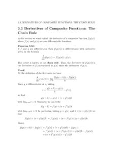
2 23 Definition of the derivative .. 26 Notations for describing change: .. 28 A slightly closer look at limits: .. 28 Rules of differentiation .. 29 Composite functions .. 32 The chain rule of differentiation .. 32 Elasticities .. 34 Increasing/decreasing functions .. 35 Inverse functions .. 37 Exponential functions and logarithmic functions .. 39 Using logarithms to simplify.. 44 The general exponential function ax, a>0 .. 45 Differentiation of composite functions involving exponentials: .. 45 PART 3 OPTIMISATION .. 46 Extreme points .. 47 Higher order derivatives .. 55 3 Convexity and concavity .. 56 Second order-conditions for maximum/minimum: .. 60 PART 4. FUNCTIONS OF MORE THAN ONE VARIABLE.

3 63 n-dimensional space .. 63 Level curves .. 63 Partial derivatives .. 66 Taking partial derivatives .. 66 The chain rule for functions of several variables and total derivatives .. 68 A special case of the chain rule .. 71 Second order conditions for a function of two variables: .. 77 Optimisation under constraints: .. 83 The Lagrange method .. 86 Reading instructions The mathematics part of the course includes lectures (6*3 hours) and exercises. The purpose of the exercises is for students to work, jointly or individually on exercises in the workbook which is available on the course webpage. During the exercise periods, the teacher is available for questions and individual tutoring. The main literature for the lectures, are these notes .

4 Sections marked * are not required. It is a good idea to have a more complete textbook for reference and to find more exercises and solved problems. There is a number of good mathematics for economists -books which you can buy or borrow from the University library. For example: Mik Wisniewski: Introductory Mathematical Methods in Economics Knut Syds ter: Matematisk analys f r ekonomer Knut Sydsaeter & Peter Hammond: Essential Mathematics for Economic Analysis Knut Sydsaeter & Peter Hammond: Mathematics for Economic Analysis R. L: Thomas: Using Mathematics in Economics Ian Jacques: Mathematics for Economics and Business Jonas M nsson: Grundl ggande matematik f r samh llsvetare och ekonomer The two last are easier to read but they do not include all the topics covered in the course.

5 4 PART 1 INTRODUCTION Why learn maths? In order to: read economic literature be able to critically assess economic theory see logical implication of assumptions discover contradictions in assumption organise Quantitative data and highlight structure isolate a particular factor But do not: o Let the mathematics take over o Take assumptions for granted o Forget that a mathematical model is no better than its assumptions o Confuse mathematical/statistical relations with causality How to learn maths? Mathematics is a science: o Learn rules and definitions precisely. o Remember the logic of the arguments. Mathematics is a craft: o Practise! Mathematics is formalised logic o It consists of deductions from assumptions - not of statements of fact and it cannot tell you anything about causality 5 6 Formal Logic: Mathematics uses implications and equivalences, sufficient conditions and necessary conditions.

6 Implication: P Q this is read as P implies Q or If P then Q where P and Q are statements. Ex 1. If (I drop the pen) then (the pen falls to the floor) This implication is true if it is not false: The implication is not true (false): If I drop the pen and it does not fall to the floor, Therefore the implication is true: If I drop the pen and it falls to the floor If I do not drop the pen and it doesn t fall to the floor. If I do not drop the pen and it falls to the floor anyway. Ex 2, If (it snows) then (it is cold outside) It snows it is cold outside. The implication is true: If it is snowing and it is cold. If it is not cold and not snowing. If it is cold and not snowing.

7 The implication is false: If it is snowing even though it isn t cold. P Q means that if P is true, then Q must always be true too. It is enough to know that P is the case to be certain that Q is the case too. When P Q, P is said to be a sufficient condition for Q. consequently the implication is false if and only if P can be true and at the same time Q is not. Example 1 is true also if I don t drop the pen and example 2 is true on a day without snow. Note the difference between saying the statement P is false and saying the implication P Q is false . 7 But if I drop the pen and it is tied by a string to my finger or if I hold my hand above a desk, the implication in example 1 is false.

8 If it snows on a warm summer day the implication in example 2 is false. P Q is the same as Not Q Not P. This means that if P is a sufficient condition for Q, then Q is always a necessary condition for P. If we know that we implication in example 2 is true we know that if it snows it is cold, but also that if it is not cold, then it is not snowing. If the temperature is +10 C, it isn t necessary to look out the window to know that it isn t snowing outside. If P Q and Q P they are said to be equivalent: P Q This is read as P (Q) is equivalent to Q (P) , P if and only if Q Example: I stand in front of the whiteboard the whiteboard is behind me Note that logical implications are not causal explanations: It snows it is cold but the snow is not the cause of or the reason for cold.

9 Economic models Elements of a model: Exogenous variables values are given, drop from the sky Endogenous variables values are determined by the model Parameters - constants (fixed numbers) in the relations that make up the model. Equations that are part of the model may have different roles. They can be: Behavioural equations Equilibrium equations (conditions) Identities Static models a snapshot of something at a given moment Comparative statics use a static model to find and compare conditions for different values of one or more exogeneous variables ( at different moments) Dynamic models show also the process of change from one condition to another 8 Example: A simple national income model Y = C + I (1) I = I0 (2) C = a + bY 0<a 0<b<1 (3) Arithmetic Real numbers and the number line The real numbers can be represented on a number line.

10 Every real number corresponds to a point on the line and every point on the line corresponds to a real number. If the point corresponding to the number A is to the left of the point corresponding to the number B on the number line, then A<B. (For example, - 1000 < - 1) The distance from a to the point zero is the absolute value of a, a The distance between a and b is a-b = b - a If a 0 then a-0 = a = a If a 0 then a = -a -(-a) = a a = -a A connected piece of the number line is called an interval. A bounded interval begins and ends in two points on the number lines. If we call the points a and b, and assume that a<b, then the closed interval [a, b] is the set of all numbers, which are equal to or larger than a and equal to or smaller than b.