Legendre Polynomials - Lecture 8 - University of Houston

1 Legendre Polynomials - Lecture 8. 1 Introduction In spherical coordinates the separation of variables for the function of the polar angle results in Legendre 's equation when the solution is independent of the azimuthal angle. 2. (1 x2 ) d P2 2x dP + l(l + 1)P = 0. dx dx This equation has x = cos( ) with solutions Pl (x). As previously demonstrated, a series solution can be obtained using the form;. an xn+s P. P (x) =. Taking the derivatives, substituting into the ode, and collecting the coefficient of the same power in x, one obtains the recursion relation for the coefficients. (n + s)(n + s + 1) l(l + 1). an+2 = an (n + s + 2)(n + s + 1). The indicial equation must also be satisfied by selection of the initial coefficient and/or start- ing power of x. Thus a0 s(s 1) = 0. a1 (1 + s)s = 0. We then have the choice of a1 = 0 and s = 0 or a0 = 0 and s = 0.

2 Other choices are incorporated in these two. Thus if we choose a1 = 0 and s = 0, then;. n(n + 1) l(l + 1). an+2 = an (n + 2)(n + 1). Only even powers of x are included in the series. If a0 and s = 0 then only odd powers are incorporated in the series and the recursion relation remains the same. For the series to be convergent for |x| = 1 it must terminate, again as previously pointed out. The series then takes the form;. l/2. (2l 2n)! ( 1)n xl 2k P. Pl (x) = l n=0 2 n!(l n)!(l 2n)! This series results in a set of Polynomials which may be obtained from the generating func- tion;. 1.. g(x, t) = (1 2xt + t2 ) 1/2 = Pl (x) tl P. l=0. Some initial Polynomials are;. P0 = 1. P1 = x P2 = (1/2)[3x2 1]. 2 Orthogonality Consider the orthogonality integral for the Legendre functions. This follows from the general Sturm-Liouville problem.

3 Put Legendre 's equation in self adjoint form;. d [(1 x2 ) dPl (x) ] + l(l + 1)P (x) = 0. l dx dx Then look at the equation for Pn (x) and subtract the equations for Pl and Pn after multipli- cation of the first by Pn and the later by Pl . Integrate the result between 1. This results in R1. [(1 x2 )Pn Pl (1 x2 )Pl Pn ]1 1 + [l(l + 1) n(n + 1)] dxPl Pn = 0. 1. The first term vanishes and thus the Polynomials are orthogonal but not normalized to 1. The normalization integral takes the form;. R1. N2 = dx Pn Pm 1. Use the Rodgiques formula to obtain;. Pn (x) = 1 ( d )n (x2 1)n 2n n! dx ( 1)m+n R1 m m N2 = m+n dx [( d m )(1 x2 )m ][( d n )(1 x2 )n ]. 2 m!n! 1 dx dx Integrate by parts m times noting that the surface terms vanish at 1. ( 1)n m R1 n m N2 = n+m dx ( d n m )(1 x2 )n 2 m!n! 1 dx 2. This vanishes for n > m (reverse n, m if n < m).

4 If n = m then;. 1 R1. N2 = 2n 2 dx (1 x2 )n = 2n 2+ 1. 2 (n!) 1. The orthogonality integral is for the associated Legendre Polynomials is expressed as;. R1 (j + m)! dx Prm (j)Pkm (x) = 2j 2+ 1. 1. (j m)! The normailzation for the Legendre polynomial Prm is found for m = 0. 3 Recurrence Relations The recurrence relations between the Legendre Polynomials can be obtained from the gen- erating function. The most important recurrence relation is;. (2n + 1)xPn (x) = (n + 1)Pn+1 (x) + nPn 1 (x). To generate higher order Polynomials , one begins with P0 (x) = 1 and P1 (x) = x. The gen- erating function also gives the recursion relation for the derivative.. Pn+1 (x) = (n + 1)Pn (x) + xPn (x). 4 Separation of variables in spherical coordinates We have previously looked at separation of variables in spherical coordinates , particularly with respect to the radial component.

5 Now consider the component involving the polar angle with x = cos( ) when the aximuthal angle id included in the separation. 2 2. (1 x2 ) d d . 2 2x dx + [n(n + 1) . m ] = 0. dx (1 x2 ). The above equation is the associated Legendre equation. For the solution to remain finite at x = 1 with n integral. The equation may be obtained from the ordinary Legendre equation by differentiation. dmm [(1 x2 )P (x) 2xP (x) + n(n + 1)P (x)]. n n n dx Thus we find;. 3. dm Pn (x). Pnm (x) = (1 x2 )m/2. dxm Then;. (n m)! m Pn m (x) = ( 1)m P (x). (n + m)! n The generating function is difficult to use;. (2m)!(1 x2 )m/2 . m (x) ts P. = Ps+m 2m m!(1 2tx + t2 )m+1/2 s=0. The recursion relation is;. (2n + 1)xPnm (x) = (n + m)Pn 1. m m (x) + (n m + 1)Pn+1 (x). Finally;. Pnm ( x) = ( 1)n+m Pnm (x). Pnm ( 1) = 0. 5 spherical harmonics In spherical coordinates Laplace's equation has the form.

6 2 V = (1/r 2) (r 2 V ) + 2 1 (sin( ) V ) + 1 2V. r r r sin( ) r sin ( ) 2. 2 2. Now identify an operator on the angles, L, such that;. (1/r 2 )L2 V = 1 (sin( ) V ) + 1 2V. 2. r sin( ) r sin ( ) 2. 2 2. Then when Laplace's equation is solved by separation of variables;. L2 V = l(l + 1)V. Thus identify V = Rl (r) Ylm ( , ) where Ylm ( , ) is an angular eigenfunction with eigenval- ues, l, and m. We already know that this function has the form;. Ylm ( , ) Plm ( ) eim . 4. Now we make this function not only orthogonal, which it must be when integrating over and , but also normalized to 1. Therefore integrating over the solid angle, d = sin( ) d d ;. R R2 . nm lk = sin( ) d d [Ylm Ykm ]. 0 0. Then;. r (2l + 1)(l m)! m Ylm ( , ) = Pl ( , ) eim . 4 (l + m)! The first few functions, YlM , which are the spherical harmonics;. p Y00 = 1/(4 ).

7 P Y11 = 3/(8 ) sin( ) ei . 1. p Y 1 = 3/(8 ) sin( ) e i . p Y01 = 3/(4 ) cos( ). Note that Ylm = Yl m . The functions, Ylm ( , ), are the spherical harmonics, and we will later identify the operator, L, as proportional to the angular momentum operator in Quantum Mechanics. 6 Second solution We have found a series solutions, Pl (x) with x = cos( ), which contain only odd powers and one containing only even powers. But while these are linearly independent, they are not the two linearly independent solutions solutions expected from a 2nd order ode. In fact, we have demonstrated that a second solution must diverge at the singular points. Suppose we choose to allow divergence by not letting the series terminate. Thus write;. = Pl + Ql In the above, Ql will be the second solution. For the series solution we look at the form.

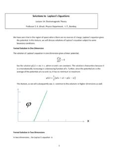
8 Bn xn P. = Pl +. n=1. Now l is chosen so that the series in even powers terminates. We then start bn with n = 1. so this series forms even powers of x which cannot terminate because l is already chosen to 5. Figure 1: A representative example of Legendre functions of the first kind make the even series terminate. The recursion relation is;. n(n + 1) l(l + 1). bn+2 = b n odd (n + 2+)(n + 1) n We can also generate a series in even powers in the same way. This series represents the second solution to Legendre 's equation and is written, Ql . Ql has singular points at = 0, . Associated functions, as with the function, Pl , are defined and written, Qm l ( ). The first few functional forms are;. Q0 = (1/2) ln[ 11 . + x]. x Q1 = (x/2) ln[ 11 . + x] 1. x 2. Q2 = ( 3x 4 1 ) ln[ 11 . + x ] 3x/2. x Figure 1 shows the behavior of the first few Legendre functions of the first kind, while Figure 2 shows the behavior of the Legendre functions of the second kind.

9 6. Figure 2: A representative example of Legendre functions of the first kind 7 Green's function in spherical coordinates Now return to the expression of the Green's function in spherical coordinates . This was developed several times previously but we are now in position to finalize this result. We assume that;. 2 G = 4 (~r ~r ). Now expand the function using the complete set of spherical harmonics. Thus;. ( ) ( ) = a Y ( ). P. Multiply by Ylm ( , ) and integrate over the solid angle d . Ortho-normality projects out the coefficients, alm = Ylm ( , ). Then the Green's function takes the form;. gl Ylm ( , ) Ylm ( , ). P. G =. lm The delta function is;. (~r ~r ) = 4 (r r ) Ylm ( , ) Ylm ( , ). P. lm Substitution into Laplaces's equation yields;. 7. 2. r d 2 [rg] l(l + 1)g = 4 (r r ). dr This is solved by requiring the solution to be continuous and the derivative to match the discontinuity at r = r.

10 The two solutions to the homogeneous equation are r l and r (l+1) . The result is;. rl . r < r . g(r, r ) = 4 r (l+1). r l . 2l + 1 . r > r r (l+1). The Green's function is then;. l G =. P 4 r< Y m ( , )Y m ( , ). lm 2l + 1 r>l+1 l l Alternatively expand the factor, 1. |~r ~r |. Choose r > r and 1 = (1/r) 1. |~r ~r | 1 (r /r) cos( ) + (r /r)2. 1 P r . = l+1 Pl (cos( )). |~r ~r | m r When comparing this to the expression for the Green's function above, it automatically gives the addition theorem. Pl (cos( )) =. P 4 m m . m 2m + 1 Yl ( , )Yl ( , ). Return to the expansion of the vector form 1 . Figure 3 shows the geometry. |~r ~r |. Apply a power series expansion in powers of r /r when r > r . 1 1. R = r[1 (r /r)cos( ) + (r /r)2 ]1/2. 1 2 2. R = (1/r) + (r /r)cos( ) + (r /r) [1/2(3cos ( ) 1)] + . 1 = P (r l l/r l+1 ) P (cos( )).