Transcription of Lesson 16 Post-hoc Tests
1 Lesson 16 Post-hoc Tests Outline Tukey s HSD Post-hoc test -differences between means -studentized range statistic (q) -honestly significant difference (HSD) Example Tukey Problem Magnitude of the Effect -eta-square -omega-square Tukey s HSD Post-hoc test A Post-hoc test is needed after we complete an ANOVA in order to determine which groups differ from each other. Do not conduct a Post-hoc test unless you found an effect (rejected the null) in the ANOVA problem. If you fail to reject the null, then there are no differences to find. For the Tukey s Post-hoc test we will first find the differences between the means of all of our groups. We will compare this difference score to a critical value to see if the difference is significant. The critical value in this case is the HSD (honestly significant difference) and it must be computed. It is the point when a mean difference becomes honestly significantly different.
2 NMSqHSDW ithin= Note that q is a table value, and n is the number of values we are dealing with in each group (not total n). The Mean Square value is from the ANOVA you already computed. To find q or the studentized range statistic, refer to your table on page A-32 of your text. On the table k or the number of groups is found along the top, and degrees of freedom within is down the side. Cross index the row and column to find the value you need to put in the formula above. Example This example is a continuation of the ANOVA problem we did in the last Lesson . Here I show the groups, but have computed the average or mean of each group. Therapy A Therapy B Therapy C 5 3 1 2 3 0 5 0 1 4 2 2 2 2 1 = =2X 2 =3X1 The first step is to compute all possible differences between means: = XX = XX = = XX We will only be concerned with the absolute difference, so, you can ignore any negative signs.
3 Next we compute HSD. nMSqHSDW ithin== = )53(. Now we will compare the difference scores we computed with the HSD value. If the difference is larger than the HSD, then we say the difference is significant. Groups 1 and 2 do not differ Groups 1 and 3 differ Groups 2 and 3 differ Magnitude of the Effect It is a common misconception that the size of the F-ratio you compute directly indicates how strongly the relationship is between the independent and dependent variable. However, a separate computation is needed to get a true idea of the strength of the relationship. Our test indicates only that there is difference in the treatments, and it is not a measure of a relationship between variables. Magnitude of the effect is the amount of variability that our independent variable can account for in the dependent variable. The easiest measure of the effect is eta-square ( 2). It measures the proportion of our between factor variability to the total variability.
4 If we know what proportion of variability of the total is due to our treatment, we will have a rough idea of how strong the relationship might be. totalBetweenSSSS=2 Notice it is just a ratio of treatment effect variability to total variability For our example: 50% of the variability in rated fear of spiders is due to the type of therapy they received. One problem with eta-square is that it is a biased estimate and tends to overestimate the effect. A more accurate measure of the effect is omega-square ( 2). ()WithintotalWithinBetweenMSSSMSkSS+ =12 () )2( = =+ =