Transcription of Linear Regression - Columbia University
1 Linear Regression In this tutorial we will explore fitting Linear Regression models using STATA. We will also cover ways of re- expressing variables in a data set if the conditions for Linear Regression aren t satisfied. We will be working with the data set discussed in examples on page 210 of the textbook. The data set consists of three variables waist (waist size in inches), weight (weight in pounds) and fat (body fat in %) measured on 20 male subjects. To access the data type: use ~martin/W1111/Data/Body_fat in the command window. To create a scatter plot for the variables fat and waist type: scatter fat waist This gives rise to the following plot: 010203040fat30354045waist Studying the plot, the association between the variables appears to be strong, Linear and positive.
2 As the scatter plot indicates a Linear relationship between the variables we decide to find the least-squares Regression line. We do this by typing the command: regress fat waist In this notation the first variable, fat, is the response variable and the second variable, waist, is the explanatory command gives rise to the following output in the results window: The output indicates that the least-square Regression line is given by. + = This implies that for each additional inch in waist size, the model predicts an increase of body fat. The fraction of the variability in fat that is explained by the least squares line of fat on waist is equal to Next, we want to calculate the predicted values from the Regression .
3 We can do this by typing: predict yhat, xb This command is solely used to create a new variable, yhat, and there will be no output in the results window. However, if you look in the variables window a new variable yhat is now present. To plot the Regression line together with the data type: scatter fat waist || line yhat waist A vertical line can be obtained by simultaneously pressing the shift and the backslash (\) button on your keyboard. This button is located directly above the enter key. To obtain two vertical lines, repeat this procedure twice. The command above tells STATA to create a scatterplot of fat against waist and superimpose the line given by yhat created in the previous command.
4 This command gives the following plot: 010203040fat/ Linear prediction30354045waistfatLinear prediction The line appears to fit the data well. However, it is important to make residual plots when performing Regression . We can calculate the residuals by typing the command: predict r, resid Again, note that other than creating a new variable, r, there will be no additional output. The new variable consists of the set of residuals, and a residual plot can be created by typing: scatter r waist This gives rise to the following plot: -10-50510 Residuals30354045waist The residual plot shows no apparent pattern. The residual plot and the relatively high value of 2R indicate that the Linear model we fit is appropriate.
5 Re- expressing Data Often the conditions necessary for performing Linear Regression aren t satisfied in a data set. However, it may still be possible to use these methods if we re-express one or both of the variables. To re-express data we need be able to create new variables using STATA. We can do this using the generate command. For example to create a new variable named logx which is the logarithm of an already existing variable x, we type: generate logx = log(x) If we instead wanted to create a variable that is the square root of x, we could type generate sqx = sqrt(x) In general, the command is on the format: generate new_variable = expression(old_variable) where expression is the mathematical function applied to the old variable.
6 Note that by default STATA uses log base e. Linear Regression using re-expressed data In this portion of the tutorial we will be working with the data set discussed in example on page 256 of the textbook. The data set gives information on the highest paid baseball players in the period spanning 1980-2001. The data set consists of 3 variables player, year and salary. To access the data type: use ~martin/W1111/Data/salary in the command window. We begin by making a scatter plot of salary and year. scatter salary year This gives rise to the following plot: 0510152025salary19801985199019952000year The relationship between year and highest salary is moderately strong, positive and curved.
7 Since the scatter plot shows a curved relationship, a Linear model is not appropriate. However, it appears that taking the logarithm of salary may help straighten the plot. We can generate a new variable named logsalary, which is the logarithm of the variable salary, by typing: generate logsalary = log(salary) We can make a scatter plot of this new variable against year by typing scatter logsalary year This gives rise to the following plot: 0123logsalary19801985199019952000year It appears that the transformation has significantly straightened the scatter plot. We can now proceed with fitting a Linear Regression model to the transformed data by typing: regress logsalary year Note that now the response variable is logsalary instead of salary.
8 This gives rise to the following output: The output indicates that the least-square Regression line is given by. ) log(+ = The fraction of the variability in log(salary) that is explained by the least squares line of log(salary) on year is equal to Next, we want to calculate the predicted values from our Regression . We can do this by typing: predict yhat, xb Note that other than creating a new variable, yhat, there will be no additional output. To plot the Regression line together with the data type: scatter logsalary year || line yhat year The command above tells STATA to create a scatterplot of logsalary against year and to superimpose the line given by yhat.
9 This command gives the following output 0123logsalary/ Linear prediction19801985199019952000yearlogsal aryLinear prediction The line appears to fit the data well. However, we always want to make sure to check the residual plots. We can calculate the residuals by typing the command: predict r, resid Again, note that other than creating a new variable named r there will be no additional output. We can use this new variable to create a residual plot by typing: scatter r year This gives rise to the following output: The residual plot shows no apparent pattern. Homework: Do problems and from the textbook. Solve both of these problems using STATA.
10 For each questions make sure to hand in (a) your log file, (b) a scatter plot with a Regression line superimposed, (c) a residual plot, and (d) answers to all the questions in the text.