LU-Factorization - University of California, Davis

1 MAT067 University of California, Davis Winter 2007. LU-Factorization Isaiah Lankham, Bruno Nachtergaele, Anne Schilling (March 12, 2007). 1 Introduction Given a system of linear equations, a complete reduction of the coe cient matrix to Reduced Row Echelon (RRE) form is far from the most e cient algorithm if one is only interested in nding a solution to the system. However, the Elementary Row Operations (EROs) that constitute such a reduction are themselves at the heart of many frequently used numerical ( , computer-calculated) applications of Linear Algebra. In the Sections that follow, we will see how EROs can be used to produce a so-called LU-Factorization of a matrix into a product of two signi cantly simpler matrices. Unlike Diagonalization and the Polar decomposition for Matrices that we've already encountered in this course, these LU Decompositions can be computed reasonably quickly for many matrices.

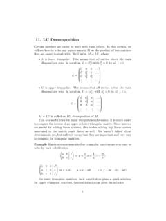
2 LU-factorizations are also an important tool for solving linear systems of equations. You should note that the factorization of complicated objects into simpler components is an extremely common problem solving technique in mathematics. , we will often factor a polynomial into several polynomials of lower degree, and one can similarly use the prime factorization for an integer in order to simply certain numerical computations. 2 Upper and Lower Triangular Matrices We begin by recalling the terminology for several special forms of matrices. A square matrix A = (aij ) Fn n is called upper triangular if aij = 0 for each pair of integers i, j {1, .. , n} such that i > j. In other words, A has the form . a11 a12 a13 a1n 0 a22 a23 a2n .. 0 a33 a3n.

3 A= 0 .. 0 0 0 ann Copyright c 2006 by the authors. These lecture notes may be reproduced in their entirety for non- commercial purposes. 2 UPPER AND LOWER TRIANGULAR MATRICES 2. Similarly, A = (aij ) Fn n is called lower triangular if aij = 0 for each pair of integers i, j {1, .. , n} such that i < j. In other words, A has the form . a11 0 0 0. a21 a22 0 0 .. 0 . A = a31 a32 a33 .. an1 an2 an3 ann Finally, we call A = (aij ) a diagonal matrix when aij = 0 for each i, j {1, .. , n} such that i = j. In other words, A is both an upper triangular matrix and a lower triangular matrix so that the only non-zero entries of A are along the diagonal ( , when i = j). Before applying triangularity to the solving of linear systems, we rst derive several useful algebraic properties of triangular matrices.

4 Theorem Let A, B Fn n be square matrices and c R be any real scalar. Then 1. A is upper triangular if and only if AT is lower triangular. 2. if A and B are upper triangular, (a) cA is upper triangular, (b) A + B is upper triangular, and (c) AB is upper triangular. 3. all properties of Part 2 hold when upper triangular is replaced by lower triangular. Proof. The proof of Part 1 follows directly from the de nitions of upper and lower triangu- larity in addition to the de nition of transpose. The proofs of Parts 2(a) and 2(b) are equally straightforward. Moreover, the proof of Part 3 follows by combining Part 1 with Part 2 but when A is replaced by AT and B by B T . Thus, we need only prove Part 2(c). To prove Part 2(c), we start from the de nition of the matrix product.

5 Denoting A = (aij ). and B = (bij ), note that AB = ((ab)ij ) is an n n matrix having i-j entry given by . n (ab)ij = aik bkj . k=1. Since A and B are upper triangular, we have that aik = 0 when i > k and that bkj = 0. when k > j. Thus, to obtain a non-zero summand aik bkj = 0, we must have both aik = 0, which implies that i k, and bkj = 0, which implies that k j. In particular, these two conditions are simultaneously satis able only when i j. Therefore, (ab)ij = 0 when i > j, from which AB is upper triangular. 3 BACK AND FORWARD SUBSTITUTION 3. As a side remark, we mention that Parts 2(a) and 2(b) of Theorem imply that the set of all n n upper triangular matrices forms a proper subspace of the vector space of all n n matrices. (One can furthermore see from Part 2(c) that the set of all n n upper triangular matrices actually forms a subalgebra of the algebra of all n n matrices.)

6 3 Back and Forward Substitution Consider an n n linear system of the form Ax = b with A an upper triangular matrix. To solve such a linear system, it is not at all necessary to rst reduce it to Reduced Row Echelon (RRE) form. To see this, note that the last equation in such a system can only involve the single unknown xn and that, moreover, bn xn =. ann as long as ann = 0. If ann = 0, then we must be careful to distinguish the two cases where bn = 0 and bn = 0. Thus, for concreteness, we assume that the diagonal elements of A are all nonzero, and so we can next substitute the solution for xn into the second-to-last equation. Since A is upper triangular, the resulting equation will involve only the single unknown xn 1 , and, moreover, bn 1 an 1,n xn xn 1 =.

7 An 1,n 1. One can then similarly substitute the solutions for xn and xn 1 into the ante penultimate equation in order to solve for xn 2 , and so on until the complete solution is found. We call this process back substitution. Note that, as an intermediate step in our algorithm for reduction to RRE form, we obtain an upper triangular matrix that is row equivalent to A. Back substitution allows one to stop the reduction at that point and solve the linear system. A similar procedure can be applied when A is lower triangular. In this case, the rst equation contains only x1 , so b1. x1 = , a11. where we are again assuming that the diagonal entries of A are all nonzero. Then, as above, we can substitute the solution for x1 into the second equation to obtain b2 a21 x1.

8 X2 = . a22. Continuing this process, we obtain the forward substitution procedure. In particular, . bn n 1. k=1 ank xk xn = . ann 4 LU FACTORIZATION 4. We next consider a more general linear system Ax = b, for which we assume that there is a lower triangular matrix L and an upper triangular matrix U such that A = LU. Such a system is more general since it clearly includes the special cases of A being either lower or upper triangular. In order to solve such a system, we can again exploit triangularity in order to produce a solution without applying a single Elementary Row Operation. To accomplish this, we rst set y = Ux, where x is the as yet unknown solution of Ax = b. Then note that y must satisfy Ly = b. As L is lower triangular, we can solve for y via forward substitution (assuming that the diagonal entries of L are all nonzero).

9 Then, once we have y, we can apply back substitution to solve for x in the system Ux = y since U is upper triangular. (As with L, we must also assume that every diagonal entry of U is nonzero.). In summary, we have given an algorithm for solving any linear system Ax = b in which we can factor A = LU, where L is lower triangular, U is upper triangular, and both L and U. have all non-zero diagonal entries. Moreover, the solution is found entirely through simple forward and back substitution, and one can easily verify that the solution obtained is unique. We note in closing that the simple procedures of back and forward substitution can also be regarded as a straightforward method for computing the inverses of lower and upper triangular matrices.

10 The only condition we imposed on our triangular matrices above was that all diagonal entries were non-zero. It should be clear to you that this non-zero diagonal restriction is a necessary and su cient condition for a triangular matrix to be non-singular. Moreover, once the inverses of L and U have been obtained, then we can immediately calculate the inverse for A by noting that A 1 = (LU) 1 = U 1 L 1 . 4 LU factorization Based upon the discussion in the previous Section, it should be clear that one can nd many uses for the factorization of a matrix A = LU into the product of a lower triangular matrix L and an upper triangular matrix U. This form of decomposition of a matrix is called an LU-Factorization (or sometimes LU- decomposition ). One can prove that such a factorization, with L and U satisfying the condition that all diagonal entries are non-zero, is equivalent to either A or some permutation of A being non-singular.