M.I.T. 18.03 Ordinary Di erential Equations

1 Differential EquationsNotes and ExercisesArthur Mattuck, Haynes Miller, David Jerison,Jennifer French, Jeremy NOTES, EXERCISES, AND Integral and Numerical Response Differential Response and Coverup and Green s Systems: Review of Linear Linear Systems with Constant and Repearted of Linear ODE and Amplitude Plane and Linear Multiplication, Rank, Solving Linear Solutions, Nullspace, Space, Dimension, and and and Orthogonal Dimensional , Normal Matrix s Theory of ; Insulated Wave EquationEXERCISES (exercises with * are not solved) Order ODE Order ODE Algebra ExercisesSOLUTIONS TO EXERCISESc A. Mattuck, Haynes Miller, David Jerison, Jennifer French 2007, 2013, 2017D. Definite Integral SolutionsYou will find in your other subjects that solutions to Ordinary differential Equations (ODE s) are often written as definite integrals, rather thanas indefinite integrals.

2 Thisis particularly true when initial conditions are given, , an initial-value problem (IVP)is being solved. It is important to understand the relation between the two forms for a simple example, consider the IVP(1)y = 6x2,y(1) = the usual indefinite integral to solve it, we gety= 2x3+c, and by substitutingx= 1, y= 5, we find thatc= 3. Thus the solution is(2)y= 2x3+ 3 However, we can also write down this answer in another form, as a definite integral(3)y= 5 + x16t2dt .Indeed, if you evaluate the definite integral, you will see right away that the solution (3) isthe same as the solution (2). But that is not the before actually integrating,youcan see that (3) solves the IVP (1). For, according to the Second Fundamental Theorem ofCalculus,ddx xaf(t)dt=f(x).If we use this and differentiate both sides of (3), we see thaty = 6x2, so that the firstpart of the IVP (1) is satisfied.

3 Also the initial condition issatisfied, sincey(1) = 5 + 116t2dt= the above example, the explicit form (2) seems preferableto the definite integral form(3). But if the indefinite integration that leads to (2) cannot be explicitly performed, wemust use the integral. For instance, the IVPy = sin(x2), y(0) = 1is of this type: there is no explicit elementary antiderivative (indefinite integral) for sin(x2);the solution to the IVP can however be written in the form (3):y= 1 + x0sin(t2)dt .The most important case in which the definite integral form (3) must be used is inscientific and engineering applications when the functionsin the IVP aren t specified, butone still wants to write down the solution explicitly. Thus,the solution to the general IVP(4)y =f(x),y(x0) =y0may be NOTES(5)y=y0+ xx0f(t)dt .If we tried to write down the solution to (4) using indefinite integration, we would have tosay something like, the solution isy= f(x)dx+c, where the constantcis determinedby the conditiony(x0) =y0 an awkward and not explicit short, the definite integral (5) gives us an explicit solution to the IVP; the indefiniteintegral only gives us a procedure for finding a solution, andjust for those cases when anexplicit antiderivative can actually be Graphical and Numerical MethodsIn studying the first-order ODE(1)dydx=f(x, y),the main emphasis is on learning different ways of finding explicit solutions.

4 But you shouldrealize that most first-order Equations cannot be solved explicitly. For such Equations , oneresorts to graphical and numerical methods . Carried out by hand, the graphical methodsgive rough qualitative information about how the graphs of solutions to (1) look geometri-cally. The numerical methods then give the actual graphs to as great an accuracy as desired;the computer does the numerical work, and plots the Graphical graphical methods are based on the construction of what is called adirection fieldfor the equation (1). To get this, we imagine that through each point (x, y) of the plane isdrawn a little line segment whose slope isf(x, y). In practice, the segments are drawn inat a representative set of points in the plane; if the computer draws them, the points areevenly spaced in both directions, forming a lattice.

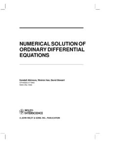
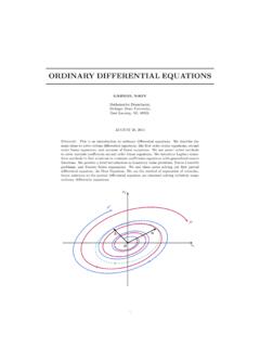
5 If drawn by hand, however, they arenot, because a different procedure is used, better adapted construct a direction field by hand, draw in lightly, or in dashed lines, what are calledtheisoclinesfor the equation (1). These are the one-parameter family of curves given bythe Equations (2)f(x, y) =c, the isocline given by the equation (2), the line segments all have the same slopec;this makes it easy to draw in those line segments, and you can put in as many as you want.(Note: iso-cline = equal slope .)The picture shows a direction field for the equationy =x y .The isoclines are the linesx y=c, two of whichare shown in dashed lines, corresponding to the valuesc= 0, 1. (Use dashed lines for isoclines).Once you have sketched the direction field for the equa-tion (1) by drawing some isoclines and drawing in littleline segments along each of them, the next step is todraw in curves which are at each point tangent to the line segment at that point.

6 Suchcurves are calledintegral curvesorsolution curvesfor the direction field. Their significanceis this:(3)The integral curves are the graphs of the solutions toy =f(x, y). the integral curveCis represented near the point (x, y) by the graph ofthe functiony=y(x). To say thatCis an integral curve is the same as saying0G. GRAPHICAL AND NUMERICAL METHODS1slope ofCat (x, y) = slope of the direction field at (x, y);from the way the direction field is defined, this is the same as sayingy (x) =f(x, y).But this last equation exactly says thaty(x) is a solution to (1). We may summarize things by saying, the direction field gives apicture of the first-orderequation (1), and its integral curves give a picture of the solutions to (1).Two integral curves (in solid lines) have been drawn for the equationy =x y. Ingeneral, by sketching in a few integral curves, one can oftenget some feeling for the behaviorof the solutions.

7 The problems will illustrate. Even when the equation can be solved exactly,sometimes you learn more about the solutions by sketching a direction field and some integralcurves, than by putting numerical values into exact solutions and plotting is a theorem about the integral curves which often helps in sketching Curve Theorem.(i) Iff(x, y)is defined in a region of thexy-plane, then integral curves ofy =f(x, y)cannot cross at a positive angle anywhere in that region.(ii) Iffy(x, y)is continuous in the region, then integral curves cannot even be tangentin that convenient summary of both statements is (here smooth = continuously differentiable):Intersection Principle(4)Integral curves ofy =f(x, y)cannot intersect whereverf(x, y)is of the first statement (i) is easy, for at any point (x0, y0) wherethey crossed, the two integral curves would have to have the same slope, namelyf(x0, y0).

8 So they cannot cross at a positive second statement (ii) is a consequence of the uniquenesstheorem for first-orderODE s; it will be taken up then when we study that theorem. Essentially, the hypothesisguarantees that through each point (x0, y0) of the region, there is a unique solution to theODE, which means there is a unique integral curve through that point. So two integralcurves cannot intersect in particular, they cannot be tangent at any point wheref(x, y) has continuous : Section NOTES2. The ODE of a family. Orthogonal solution to the ODE (1) is given analytically by anxy-equation containing anarbitrary constantc; either in the explicit form (5a), or the implicit form (5b):(5)(a)y=g(x, c)(b)h(x, y, c) = either form, as the parameterctakes on different numerical values, the correspondinggraphs of the Equations form a one-parameter family of curves in now want to consider the inverse problem.

9 Starting with anODE, we got a one-parameter family of curves as its integral curves. Suppose instead we start with a one-parameter family of curves defined by an equation of the form (5a) or (5b), can we find afirst-order ODE having these as its integral curves, theequations (5) as its solutions?The answer is yes; the ODE is found by differentiating the equation of the family (5)(using implicit differentiation if it has the form (5b)), andthen using (5) to eliminate thearbitrary constantcfrom the differentiated a first-order ODE whose general solution is the family(6)y=cx c(cis an arbitrary constant). differentiate both sides of (6) with respect tox, gettingy = c(x c) eliminatecfrom this equation, in steps. By (6),x c=c/y, so that(7)y = c(x c)2= c(c/y)2= y2c;To get rid ofc, we solve (6) algebraically forc, gettingc=yxy+ 1; substitute this for thecon the right side of (7), then cancel ayfrom the top and bottom; you get as the ODEhaving the solution (6)(8)y = y(y+ 1) not appear in the ODE, since then we would not have a single ODE,but rather a one-parameter family of ODE s one for each possible value ofc.

10 Instead, wewant just one ODE which has each of the curves (5) as an integral curve, regardless of thevalue ofcfor that curve; thus the ODE cannot itself a one-parameter family of plane curves, itsorthogonal trajectoriesare anotherone-parameter family of curves, each one of which is perpendicular to all the curves in theoriginal family. For instance, if the original family consisted of all circles having center atthe origin, its orthogonal trajectories would be all rays (half-lines) starting at the trajectories arise in different contexts in applications. For example, if theoriginal family represents thelines of forcein a gravitational or electrostatic field, its or-thogonal trajectories represent theequipotentials, the curves along which the gravitationalor electrostatic potential is GRAPHICAL AND NUMERICAL METHODS3In a temperature map of the , the original family would betheisotherms, the curvesalong which the temperature is constant; their orthogonal trajectories would be thetem-perature gradients, the curves along which the temperature is changing most generally, if the original family is of the formh(x, y) =c, it represents thelevelcurvesof the functionh(x, y).