Transcription of METHODOLOGY AND APPLICATIONS OF …
1 METHODOLOGY AND APPLICATIONS OF. stochastic frontier analysis . Andrea Furkov . STRUCTURE OF THE PRESENTATION. Part 1. Theory: Illustration the basics of stochastic frontier analysis (SFA). Concept of efficiency Estimation Identification of sources of inefficiency Part 2. An APPLICATIONS of SFA. Theory usually presents the producers as successful optimizers. They maximize production, minimize cost, and maximize profits. Conventional econometric techniques build on this base to estimate production/cost/profit function parameters using regression techniques where deviations of observed choices from optimal ones are modeled as statistical noise. Econometric estimation techniques should allow for the fact that deviations of observed choices from optimal ones are due to two factors: failure to optimize , inefficiency due to random shocks.
2 stochastic frontier analysis is one such technique to model producer behavior. Methods based on efficient frontier Based on benchmarking, that is, a unit's performance is compared with a reference performance (so-called efficient frontier ). Unit's inefficiency can results from technological deficiencies (technical inefficiency) or non- optimal allocation of resources into production (allocative inefficiency). Both technical and allocative inefficiencies are included in cost (economic) inefficiency. Generally, there are two families of methods based on efficient frontier : Non-parametric methods, like Data Envelopment analysis (DEA) or Free Disposal Hull (FDH).
3 These methods originate from operations research and use linear programming to calculate an efficient deterministic frontier against which units are compared. Parametric methods, like stochastic frontier analysis (SFA), Thick frontier Approach (TFA) and Distribution Free Approach (DFA). Econometric theory is used to estimate pre-specified functional form and inefficiency is modeled as an additional stochastic term. stochastic frontier analysis time invariant efficiency Based on econometric theory and pre-specified functional form is estimated and inefficiency is modeled as an additional stochastic term. The stochastic frontier production function model (single Cobb-Douglas form for panel data): ln y it = 0 + n ln x nit + v it u i i = 1.
4 ,N t = 1,..,T. it = vit ui n ui 0. yit - observed output quantities of the i-th unit in year t, xit - observed inputs quantities of the i-th unit in year t, ui - non negative time-invariant random variables capturing time-invariant technical inefficiency, vit - random variables of i-th unit in year t reflecting effect of statistical noise frontier cost function: identifies the minimum costs at a given output level, input prices and existing production technology stochastic frontier cost function model (single Cobb- Douglas form for panel data): ln C it = 0 + y ln y it + n ln w nit + v it + u i ui 0. it = vit + ui n i = 1,..,N t = 1,..,T. Cit - observed total costs of the i-th unit in year t, yit - a vector of outputs of the i-th unit in year t, wit - an input price vector of the i-th unit in year t, ui - time-invariant cost inefficiency, vit - random variables of i-th unit in year t reflecting effect of statistical noise SPECIFICATION OF THE MODEL.
5 1. Deterministic kernel of the model Cobb-Douglas (in log form). Translog (a flexible functional form). 2. Estimation of the model Maximum likelihood estimation (ML). Generalised Least Squares method (GLS). Method of moments (MM). 3. Calculating unit s specific efficiency Maximum likelihood estimation (ML). Distribution assumptions: ui ~ iidN+ (0, u2 ) or ui ~ iidN ( , u ), vit ~ iidN(0, v2 ). + 2. Maximization of the log likelihood function The individual estimates of the technical (cost). inefficiency: JLMS decomposition - the conditional distribution of ui , conditional mean E (u i it ) or conditional modus M (u i it ) of this distribution can be used as a point estimator for ui The individual estimates of the technical (cost).
6 Efficiency: . TE i = exp E (u i | it ) .. Analyzing Efficiency Behavior Two questions: What is the behavior of efficiencies over time? Are they increasing, decreasing or constant? What explains the variations in inefficiencies among units and across time? Time behavior of inefficiencies Assumption: u it = u i + t Model: ln y it = 0 t + . n n ln x nit + v it u it i = 1,.., N t = 1,.., T. Cornwell, Schmidt and Sickles, Lee and Schmidt, Kumbhakar, Battese and Coelli Battese and Coelli proposed a simple model that can be used to estimate the time behavior of inefficiencies: u it = exp { (t T )}u i u where i ~ iidN +. ( , 2. u ) and is a parameter to be estimated.
7 Inefficiencies in periods prior to T depend on the parameter . Efficiency behavior is monotonic and ordering of units in terms of inefficiencies time-invariant. Good for understanding aggregative behavior. Explaining efficiency Certain factors influence the environment in which production takes place degree of competitiveness, input and output quality, network characteristics, ownership form, regulation etc. Two ways to handle them Include them as variables in the production process as control variables. Using this interpretation, these variables influence the structure of the technology by which conventional inputs are converted into outputs, but not efficiency.
8 Associate variation in estimated efficiency with variation in the exogenous variables. Battese a Coelli Inefficiencies are assumed to be a function of a set of explanatory variables associated with inefficiency of units over time : u it = z Tit + w it where z it - vector of variables which may influence the efficiency of units - vector of unknown parameters to be estimated 2. w it~ iid N (0, w ) random variables reflecting effect of statistical noise uit ~ iid N+(z Tit , u2). EMPIRICAL APPLICATIONS . 1. REGULATION OF DISTRIBUTION UTILITIES. Benchmarking analysis can be used by regulator as an additional instrument to establish a larger informational basis for more effective price cap regulation Incentive price cap regulation ( X efficiency factor).
9 Regulation of Slovak and Czech electricity distribution utilities Based on incentive price - cap regulation Main issue: How to set efficiency factor X, cost efficiency prediction Data: Panel data set (55 observations) for 3 Slovak and 8. Czech electricity distribution utilities over the 2000 . 2004 period Cost function specifications (Cobb-Douglas form) : Time invariant cost efficiency (estimation method ML, GLS): C PK PL . ln = 0 + Y lnYit + K ln + L ln + CUD lnCUDit + vit + ui PP it PP it PP it i = 1,.., N t = 1,.., T. Time varying cost efficiency (estimation method ML): C PK PL . ln = 0 + Y lnYit + K ln + L ln + CUD lnCUDit + vit + uit PP it PP it PP it i = 1.
10 , N t = 1,.., T. where C represents total costs, Y is the output, PK, PL, PP. are the prices of capital, labor and input purchased energy respectively, CUD is customer density Input prices labor price (PL) the average annual salary of utility . employees capital price (PK) the ratio of capital expenses to the total installed capacity of the utility's transformers in MVA. purchased energy price (PP) average price of purchased energy from generator Output variable: total output (Y) - measured as the total number of delivered electricity in MWh 2. COST EFFICIENCY ESTIMATION OF THE. BANKING SECTOR. The efficiency measuring and relative efficiency comparison of banks are crucial questions for analysts as well as for economic policy creators.