Transcription of MT-001: Taking the Mystery out of the Infamous …
1 MT-001. TUTORIAL. Taking the Mystery out of the Infamous formula , "SNR = + ," and Why You Should Care by Walt Kester INTRODUCTION. You don't have to deal with ADCs or DACs for long before running across this often quoted formula for the theoretical signal-to-noise ratio (SNR) of a converter. Rather than blindly accepting it on face value, a fundamental knowledge of its origin is important, because the formula encompasses some subtleties which if not understood can lead to significant misinterpretation of both data sheet specifications and converter performance. Remember that this formula represents the theoretical performance of a perfect N-bit ADC. You can compare the actual ADC SNR with the theoretical SNR and get an idea of how the ADC stacks up. This tutorial first derives the theoretical quantization noise of an N-bit analog-to-digital converter (ADC). Once the rms quantization noise voltage is known, the theoretical signal-to-noise ratio (SNR) is computed. The effects of oversampling on the SNR are also analyzed.
2 QUANTIZATION NOISE MODEL. The maximum error an ideal converter makes when digitizing a signal is LSB as shown in the transfer function of an ideal N-bit ADC (Figure 1). The quantization error for any ac signal which spans more than a few LSBs can be approximated by an uncorrelated sawtooth waveform having a peak-to-peak amplitude of q, the weight of an LSB. Another way to view this approximation is that the actual quantization error is equally probable to occur at any point within the range q. Although this analysis is not precise, it is accurate enough for most applications. DIGITAL. OUTPUT. ANALOG. INPUT. q = 1 LSB. ERROR. (INPUT OUTPUT). Figure 1: Ideal N-bit ADC Quantization Noise , 10/08, WK Page 1 of 7. MT-001. W. R. Bennett of Bell Laboratories analyzed the actual spectrum of quantization noise in his classic 1948 paper (Reference 1). With the simplifying assumptions previously mentioned, his detailed mathematical analysis simplifies to that of Figure 1. Other significant papers and books on converter noise followed Bennett's classic publication (References 2-6).
3 The quantization error as a function of time is shown in more detail in Figure 2. Again, a simple sawtooth waveform provides a sufficiently accurate model for analysis. The equation of the sawtooth error is given by e(t) = st, q/2s < t < +q/2s. Eq. 1. The mean-square value of e(t) can be written: 2 s + q / 2s 2. q q / 2s e (t) = (st ) dt . Eq. 2. Performing the simple integration and simplifying, 2 q2. e (t) = . Eq. 3. 12. The root-mean-square quantization error is therefore 2 q rms quantization noise = e ( t ) = . Eq. 4. 12. e(t). +q 2. SLOPE = s t q 2. q +q 2s 2s Figure 2: Quantization Noise as a Function of Time The sawtooth error waveform produces harmonics which extend well past the Nyquist bandwidth of dc to fs/2. However, all these higher order harmonics must fold (alias) back into the Nyquist bandwidth and sum together to produce an rms noise equal to q/ 12. As Bennett points out (Reference 1), the quantization noise is approximately Gaussian and spread more or less uniformly over the Nyquist bandwidth dc to fs/2.
4 The underlying assumption Page 2 of 7. MT-001. here is that the quantization noise is uncorrelated to the input signal. Under certain conditions where the sampling clock and the signal are harmonically related, the quantization noise becomes correlated, and the energy is concentrated in the harmonics of the signal however, the rms value remains approximately q/ 12. The theoretical signal-to-noise ratio can now be calculated assuming a full-scale input sinewave: q2 N. Input FS Sinewave = v ( t ) = sin(2 ft ). Eq. 5. 2. The rms value of the input signal is therefore q2 N. rms value of FS input = . Eq. 6. 2 2. The rms signal-to-noise ratio for an ideal N-bit converter is therefore rms value of FS input SNR = 20 log10 Eq. 7. rms value of quantization noise q2 N / 2 2 N 3. SNR = 20 log10 = 20 log10 2 + 20 log10 Eq. 8. q / 12 2. SNR = + , over the dc to fs/2 bandwidth. Eq. 9. Bennett's paper shows that although the actual spectrum of the quantization noise is quite complex to analyze, the simplified analysis which leads to Eq.
5 9 is accurate enough for most purposes. However, it is important to emphasize again that the rms quantization noise is measured over the full Nyquist bandwidth, dc to fs/2. FREQUENCY SPETRUM OF QUANTIZATION NOISE. In many applications, the actual signal of interest occupies a smaller bandwidth, BW, which is less than the Nyquist bandwidth (see Figure 3). If digital filtering is used to filter out noise components outside the bandwidth BW, then a correction factor (called process gain) must be included in the equation to account for the resulting increase in SNR as shown in Eq. 10. fs SNR = N + dB + 10 log10 , over the bandwidth BW. Eq. 10. 2 BW. The process of sampling a signal at a rate which is greater than twice its bandwidth is referred to as oversampling. Oversampling in conjunction with quantization noise shaping and digital filtering are the key concepts in sigma-delta converters, although oversampling can be used with any ADC architecture. Page 3 of 7. MT-001.
6 NOISE q SPECTRAL RMS VALUE = q = 1 LSB. DENSITY 12. fs MEASURED OVER DC TO. 2. q / 12. fs / 2. fs BW. 2. fs SNR = + + 10log10 FOR FS SINEWAVE. 2 BW. Process Gain Figure 3: Quantization Noise Spectrum Showing Process Gain The significance of process gain can be seen from the following example. In many digital basestations or other wideband receivers the signal bandwidth is composed of many individual channels, and a single ADC is used to digitize the entire bandwidth. For instance, the analog cellular radio system (AMPS) in the consists of 416 30-kHz wide channels, occupying a bandwidth of approximately MHz. Assume a 65-MSPS sampling frequency, and that digital filtering is used to separate the individual 30-kHz channels. The process gain due to oversampling for these conditions is given by: fs 65 106. Process Gain = 10 log10 = 10 log10 = dB . Eq. 11. 2 BW 2 30 103. The process gain is added to the ADC SNR specification to yield the SNR in the 30-kHz bandwidth. In the above example, if the ADC SNR specification is 65 dB (dc to fs/2), then it is increased to dB in the 30-kHz channel bandwidth (after appropriate digital filtering).
7 Figure 4 shows an application which combines oversampling and undersampling. The signal of interest has a bandwidth BW and is centered around a carrier frequency fc. The sampling frequency can be much less than fc and is chosen such that the signal of interest is centered in its Nyquist zone. Analog and digital filtering removes the noise outside the signal bandwidth of interest, and therefore results in process gain per Eq. 10. Page 4 of 7. MT-001. ZONE 1 ZONE 3. BW. fs 2fs 3fs fc fs SNR = + + 10log10 FOR FS SINEWAVE. 2 BW. Process Gain Figure 4: Undersampling and Oversampling Combined Results in Process Gain CORRELATION BETWEEN QUANTIZATION NOISE AND INPUT. T SIGNAL YIELDS. MISLEADING RESULTS. Although the rms value of the noise is accurately approximated by q/ 12, its frequency domain content may be highly correlated to the ac-input signal under certain conditions. For instance, there is greater correlation for low amplitude periodic signals than for large amplitude random signals.
8 Quite often, the assumption is made that the theoretical quantization noise appears as white noise, spread uniformly over the Nyquist bandwidth dc to fs/2. Unfortunately, this is not true in all cases. In the case of strong correlation, the quantization noise appears concentrated at the various harmonics of the input signal, just where you don't want them. In most practical applications, the input to the ADC is a band of frequencies (always summed with some unavoidable system noise), so the quantization noise tends to be random. In spectral analysis applications (or in performing FFTs on ADCs using spectrally pure sinewaves as inputs, however, the correlation between the quantization noise and the signal depends upon the ratio of the sampling frequency to the input signal. This is demonstrated in Figure 5, where the output of an ideal 12-bit ADC is analyzed using a 4096-point FFT. In the left-hand FFT plot (A), the ratio of the sampling frequency ( MSPS) to the input frequency ( MHz) was chosen to be exactly 40, and the worst harmonic is about 77 dB below the fundamental.)
9 The right hand diagram (B) shows the effects of slightly offsetting the input frequency to MHz, showing a relatively random noise spectrum, where the SFDR is now about 93 dBc and is limited by the spikes in the noise floor of the FFT. In both cases, the rms value of all the noise components is approximately q/ 12 (yielding a theoretical SNR of 74 dB) but in the first case, the noise is concentrated at harmonics of the fundamental because of the correlation. Page 5 of 7. MT-001. (A) CORRELATED NOISE (B) UNCORRELATED NOISE. fS = MSPS, fIN = MHz fS = MSPS, fIN = MHz 0 0. SFDR = 77 dBc SFDR = 93 dBc 50 50. SNR = 74 dBc SNR = 74 dBc 100 100. 150 150. 200 200. 0 5 10 15 20 25 30 35 40 0 5 10 15 20 25 30 35 40. FREQUENCY - MHz FREQUENCY - MHz Figure 5: Effect of Ratio of Sampling Clock to Input Frequency on Quantization Noise Frequency Spectrum for Ideal 12-bit ADC, 4096-Point FFT. (A) Correlated Noise, (B) Uncorrelated Noise Note that this variation in the apparent harmonic distortion of the ADC is an artifact of the sampling process caused by the correlation of the quantization error with the input frequency.
10 In a practical ADC application, the quantization error generally appears as random noise because of the random nature of the wideband input signal and the additional fact that there is a usually a small amount of system noise which acts as a dither signal to further randomize the quantization error spectrum. It is important to understand the above point, because single-tone sinewave FFT testing of ADCs is one of the universally accepted methods of performance evaluation. In order to accurately measure the harmonic distortion of an ADC, steps must be taken to ensure that the test setup truly measures the ADC distortion, not the artifacts due to quantization noise correlation. This is done by properly choosing the frequency ratio and sometimes by summing a small amount of noise (dither) with the input signal. The exact same precautions apply to measuring DAC. distortion with an analog spectrum analyzer. SNR, PROCESS GAIN, AND FFT NOISE FLOOR RELATIONSHIPS. Figure 6 shows the FFT output for an ideal 12-bit ADC.