Transcription of Multivariate Regression Modeling for Home Value …
1 Multivariate Regression Modeling for HomeValue Estimates with evaluation usingMaximum information CoefficientGongzhu Hu, Jinping Wang, and Wenying FengAbstractPredictive Modeling is a statistical data mining approach that builds aprediction function from the observed data. The function is then used to estimate avalue of a dependent variable for new data. A commonly used predictive modelingmethod is Regression that has been applied to a wide range of application this paper, we build Multivariate Regression models of home prices using a datasetcomposed of 81 homes. We then applied the maximum information coefficient(MIC) statistics to the observed home values (Y) and the predicted values (X) asan evaluation of the Regression models. The results showed very high strength of therelationship between the two words:Predictive Modeling , Multivariate linear Regression , hedonic pricemodel, maximum information IntroductionPredictive Modeling is a very commonly used method for estimating (or predicting)the outcome of an input data based on the knowledge obtained from a previousdata set.
2 It is to build a model ( functionf) from an observed data setDsuchthat the model will predict the outcome of a new inputxasf(x)with the bestGongzhu HuDepartment of Computer Science, Central Michigan University, Mt. Pleasant, MI 48859, WangGraduate Biomedical Sciences, University of Alabama at Birmingham, Birmingham, FengDepartments of Computing & information Systems and Mathematics, Trent University,Peterborough, Ontario, Canada, K9J 7B8. The domain ofxis a set ofpredictorsor independent variables, whilethe outcome is a dependent variable. Various methods have been developed forpredictive Modeling , among them, Multivariate linear Regression is perhaps oneof the most commonly used and relatively easy to build.
3 The Multivariate linearregression model is to express the dependent variableyas a linear function ofppredictor variablesxi(i=1,..,p) and an error term :y=c0+c1x1+ +cpxp+ Note that if the the relationship between the dependent variable and the predictorvariables is non-linear, we can create new variables for the non-linear terms and theregression model. For example, we can havey=c0+c1x1+c2z2+c3z3+ wherez2=x22andz3=lnx3. The linearity is actually between the dependent variableyand the a set ofndata observationsx, the linear Regression model can be expressedin matrix form:y=cX+eThe model is estimated by the least square measure that yields the coefficientscsuch that the predicted Value y=cXhas the minimal sum of the squares of the errorse=|y y|.Predictive Modeling has been widely used in many application areas, frombusiness, economy, to social and natural sciences.
4 In this paper, we apply multi-variate linear Regression to a specific economics application estimating values ofresidential homes. This is not a new problem, neither is the Regression method forsolving the problem. The novel idea presented in this paper is to use the maximuminformation coefficient (MIC) [12], which is a new statistical measure published justa few months ago, to evaluate the Regression models created. The MIC scores of thedata set we used for the experiment showed that the Regression models do have avery strong relationship with the observed home values. At the time of writing thispaper, we are not aware of any published work using MIC as an evaluation measurefor predictive Estimate of home ValuesHome values are influenced by many factors. Basically, there are two major aspects: The environmental information , including location, local economy, schooldistrict, air quality, etc.
5 The characteristics information of the property, such as lot size, house size andage, number of rooms, heating / AC systems, garage, and so people consider buying homes, usually the location has been constrainedto a certain area such as not too far from the work place. With location factor prettymuch fixed, the property characteristics information weights more in the homeprices. There are many factors describing the condition of a house, and they do notweigh equally in determining the home Value . In this paper, we present a modelingprocess for estimating home values using Multivariate linear Regression model basedon the condition information of the dwellings in order to examine the key factorseffecting their values. We also provide a general idea of figuring out if a transactionis a good deal based on the information on home prices have been going on for many years using various traditional and standard model is thehedonic pricing modelthat says the pricesof goods are directly influenced by external or environmental factors in additionto the characteristics of the goods.
6 For housing market analysis, the hedonic pricemodel [9] infers that the price of dwellings is determined by the internal factors(characteristics of the property) as well as external attributes. The method used inthis model is hedonic Regression that considers various combinations of internaland external predictors [1, 4, 13]. The predictors may be first-order or higher order(such asArea2) so that the hedonic Regression may be a polynomial function of thepredictors [2, 7].The Regression method used in our work is in fact a variation of hedonicregression, except that we did not consider external factors in our Modeling (thedata set does not include such information ). We did, however, consider differentcombinations of first-order and second-order attributes in the Regression model.
7 Theattributes are given in Table 1, whereValueis the dependent variable to be predicted,and the other are predictors including 11 first-order and 4 second-order given data set contains 81 Building of Regression Best Subsets ProcedureSince there are quite a few attributes of home condition, best subsets analysis [8]was first performed to select the best indicators to build the appropriate model. Thisprocedure finds best models with 1, 2, 3, and up to allnvariables based on the 2statistics. The Minitab output of the analysis is shown in Table on the rule that second order indicators cannot exist without first orderindicators, the impossible models were marked out in gray shade and would not beconsidered for the further analysis. Three potential cases were selected based on thehighest R-sq(adj), lowest Mallows Cp, and smallest S.
8 These three cases are coloredin Table 1 Attributes of a HouseVariableDescriptionDependentValueAs sessed home valuePredictorfirst-orderAcreageArea of lot in acresStoriesNumber of storiesAreaArea in square footageExteriorExterior condition, 1 = good / excellent, 0 = average / belowNatGes1 = natural gas heating system, 0 = other heating systemRoomsTotal number of roomsBedroomsNumber of bedroomsFullBathNumber of full bathroomsHalfBathNumber of half bathroomsFireplace1 = with, 0 = withoutGarage1 = with, 0 = withoutsecond-orderArea**2 House area squaredAcreage**2 Lot size squaredStories**2 Number of stories squaredRooms**2 Number of rooms squaredTable 2 Best subsets analysis of the variables(Shaded rows are impossible and ignored. Rows in color are selected for Modeling )Vars R-Sq R-Sq (adj) Mallows Cp SAcreageStoriesAreaExteriorNetgasRoomsBe droomsFullbathHalfbathFireplaceGarageAre a**2 Acreage**2 Stories**2 Roos**21 54006 42748 X 37902 X X 35842 X X X 34226 X X X X X5 34352 X X X X X6 33303 X X X X X 30992 X X X X X X X X X X X X X X Regression modelBased on the Best Subsets analysis results, three Regression models were built forthe three selected cases.
9 V1= 104582+45216 Acreage+36542 Stories+ +12242 FullBath+16428 Hal fBath+30480 Garage 4397 Acreage2(M-1) V2= 101097+21512 Acreage+38141 Stories+ +18580 Exterior+12218 FullBath+14569 Hal fBath+23999 Garage(M-2) V3= 111721+42939 Acreage+38965 Stories+ +18901 Exterior 6781 Rooms+12139 Bedrooms+9721 FullBath+21047 Hal fBath+24095 Garage 3919 Acreage2(M-3)Notice that the third model (M-3) has fewer variables than as indicated inthe rowVars=14of Table 2. This is because several non-significant indicatorswere removed (in the order of first removing least significant and second-orderindicators).The residuals versus fits plots for the three models are shown in Fig. 1, Fig. 2 andFig. 3, 100 50050100 Predicted Value (in thousand)Residual (in thousand)Fig.
10 1 Residuals versus fits plot of Model (M-1)The figures show a fan-shaped pattern indicating that the diagnosis analysisrevealed non-constant residual variances (residual error is not normally distributed),which is unacceptable. To alleviate the heterogeneity in the residual errors, a Box-Cox transform is applied to the dependent 100 50050100 Predicted Value (in thousand)Residual (in thousand)Fig. 2 Residuals versus fits plot of Model (M-2)0100200300400 100 50050100 Predicted Value (in thousand)Residual (in thousand)Fig. 3 Residuals versus fits plot of Model (M-3) Box-Cox TransformThe Box-Cox procedure [3] provides a suggestion of the transformation ony:y ={(y 1)/ if 6=0log if =0 After the transformation, the Box-Cox plot ( versus standard deviation) is shownin Fig.}