Transcription of Network Models 8 - Massachusetts Institute of Technology
1 Network Models 8. There are several kinds of linear-programming Models that exhibit a special structure that can be exploited in the construction of efficient algorithms for their solution. The motivation for taking advantage of their structure usually has been the need to solve larger problems than otherwise would be possible to solve with existing computer Technology . Historically, the first of these special structures to be analyzed was the trans- portation problem, which is a particular type of Network problem. The development of an efficient solution procedure for this problem resulted in the first widespread application of linear programming to problems of industrial logistics.
2 More recently, the development of algorithms to efficiently solve particular large-scale systems has become a major concern in applied mathematical programming. Network Models are possibly still the most important of the special structures in linear programming. In this chapter, we examine the characteristics of Network Models , formulate some examples of these Models , and give one approach to their solution. The approach presented here is simply derived from specializing the rules of the simplex method to take advantage of the structure of Network Models . The resulting algorithms are extremely efficient and permit the solution of Network Models so large that they would be impossible to solve by ordinary linear-programming procedures.
3 Their efficiency stems from the fact that a pivot operation for the simplex method can be carried out by simple addition and subtraction without the need for maintaining and updating the usual tableau at each iteration. Further, an added benefit of these algorithms is that the optimal solutions generated turn out to be integer if the relevant constraint data are integer. THE GENERAL Network -FLOW PROBLEM. A common scenario of a Network -flow problem arising in industrial logistics concerns the distribution of a single homogeneous product from plants (origins) to consumer markets (destinations). The total number of units produced at each plant and the total number of units required at each market are assumed to be known.
4 The product need not be sent directly from source to destination, but may be routed through intermediary points reflecting warehouses or distribution centers. Further, there may be capacity restrictions that limit some of the shipping links. The objective is to minimize the variable cost of producing and shipping the products to meet the consumer demand. The sources, destinations, and intermediate points are collectively called nodes of the Network , and the transportation links connecting nodes are termed arcs. Although a production/distribution problem has been given as the motivating scenario, there are many other applications of the general model.
5 Table indicates a few of the many possible alternatives. A numerical example of a Network -flow problem is given in Fig The nodes are represented by numbered circles and the arcs by arrows. The arcs are assumed to be directed so that, for instance, material can be sent from node 1 to node 2, but not from node 2 to node 1. Generic arcs will be denoted by i j, so that 4 5 means the arc from node 4 to node 5. Note that some pairs of nodes, for example 1 and 5, are not connected directly by an arc. 227. 228 Network Models Table Examples of Network Flow Problems Urban Communication Water transportation systems resources Product Buses, autos, etc.
6 Messages Water Nodes Bus stops, Communication Lakes, reservoirs, street intersections centers, pumping stations relay stations Arcs Streets (lanes) Communication Pipelines, canals, channels rivers Figure exhibits several additional characteristics of Network flow problems. First, a flow capacity is assigned to each arc, and second, a per-unit cost is specified for shipping along each arc. These characteristics are shown next to each arc. Thus, the flow on arc 2 4 must be between 0 and 4 units, and each unit of flow on this arc costs $ The 's in the figure have been used to denote unlimited flow capacity on arcs 2 3. and 4 5. Finally, the numbers in parentheses next to the nodes give the material supplied or demanded at that node.
7 In this case, node 1 is an origin or source node supplying 20 units, and nodes 4 and 5 are destinations or sink nodes requiring 5 and 15 units, respectively, as indicated by the negative signs. The remaining nodes have no net supply or demand; they are intermediate points, often referred to as transshipment nodes. The objective is to find the minimum-cost flow pattern to fulfill demands from the source nodes. Such problems usually are referred to as minimum-cost flow or capacitated transshipment problems. To transcribe the problem into a formal linear program, let xi j = Number of units shipped from node i to j using arc i j. Then the tabular form of the linear-programming formulation associated with the Network of Fig.
8 Is as shown in Table The first five equations are flow-balance equations at the nodes. They state the conservation-of-flow law, . Flow out Flow into Net supply = . of a node a node at a node As examples, at nodes 1 and 2 the balance equations are: x12 + x13 = 20. x23 + x24 + x25 x12 = 0. It is important to recognize the special structure of these balance equations. Note that there is one balance equation for each node in the Network . The flow variables xi j have only 0, +1, and 1 coefficients in these Figure Minimum-cost flow problem. Special Network Models 229. Table Tableau for Minimum-Cost Flow Problem Righthand x12 x13 x23 x24 x25 x34 x35 x45 x53 side Node 1 1 1 20.
9 Node 2 1 1 1 1 0. Node 3 1 1 1 1 1 0. Node 4 1 1 1 5. Node 5 1 1 1 1 15. Capacities 15 8 4 10 15 5 4. Objective function 4 4 2 2 6 1 3 2 1 (Min). equations. Further, each variable appears in exactly two balance equations, once with a +1 coefficient, corresponding to the node from which the arc emanates; and once with a 1 coefficient, corresponding to the node upon which the arc is incident. This type of tableau is referred to as a node arc incidence matrix; it completely describes the physical layout of the Network . It is this particular structure that we shall exploit in developing specialized, efficient algorithms. The remaining two rows in the table give the upper bounds on the variables and the cost of sending one unit of flow across an arc.
10 For example, x12 is constrained by 0 x12 15 and appears in the objective function as 2x12 . In this example the lower bounds on the variables are taken implicitly to be zero, although in general there may also be nonzero lower bounds. This example is an illustration of the following general minimum-cost flow problem with n nodes: XX. Minimize z = ci j xi j , i j subject to: X X. xi j xki = bi (i = 1, 2, .. , n), [Flow balance]. j k li j x i j u i j . [Flow capacities]. The summations are taken only over the arcs in the Network . That is, the first summation in the ith flow- balance equation is over all nodes j such that i j is an arc of the Network , and the second summation is over all nodes k such that k i is an arc of the Network .