Transcription of Non-Parametric Estimation in Survival Models
1 Non-Parametric Estimation in Survival Models Germ an Rodr guez Spring, 2001; revised Spring 2005. We now discuss the analysis of Survival data without parametric assump- tions about the form of the distribution. 1 One Sample: Kaplan-Meier Our first topic is Non-Parametric Estimation of the Survival function. If the data were not censored, the obvious estimate would be the empirical Survival function n = 1. X. S(t) I{ti > t}, n i=1. where I is the indicator function that takes the value 1 if the condition in braces is true and 0 otherwise. The estimator is simply the proportion alive at t. Estimation with Censored Data Kaplan and Meier (1958) extended the estimate to censored data. Let t(1) < t(2) < .. < t(m). denote the distinct ordered times of death (not counting censoring times).
2 Let di be the number of deaths at t(i) , and let ni be the number alive just before t(i) . This is the number exposed to risk at time t(i) . Then the Kaplan- Meier or product limit estimate of the survivor function is Y di . =. S(t) 1 . i:t(i) <t ni A heuristic justification of the estimate is as follows. To survive to time t you must first survive to t(1) . You must then survive from t(1) to t(2) given 1. that you have already survived to t(1) . And so on. Because there are no deaths between t(i 1) and t(i) , we take the probability of dying between these times to be zero. The conditional probability of dying at t(i) given that the subject was alive just before can be estimated by di /ni . The conditional probability of surviving time t(i) is the complement 1 di /ni.
3 The overall unconditional probability of surviving to t is obtained by multiplying the conditional probabilities for all relevant times up to t. The Kaplan-Meier estimate is a step function with discontinuities or jumps at the observed death times. Figure 1 shows Kaplan-Meier estimates for the treated and control groups in the famous Gehan data (see Cox, 1972. or Andersen et al., 1993, p. 22-23). 0 5 10 15 20 25 30 35. Figure 1: Kaplan-Meier Estimates for Gehan Data If there is no censoring, the K-M estimate coincides with the empirical Survival function. If the last observation happens to be a censored case, as is the case in the treated group in the Gehan data, the estimate is undefined beyond the last death. 2.
4 Non-Parametric Maximum Likelihood The K-M estimator has a nice interpretation as a Non-Parametric maximum likelihood estimator (NPML). A rigorous treatment of this notion is beyond the scope of the course, but the original article by K-M provides a more intuitive approach. We consider the contribution to the likelihood of cases that die or are censored at time t. If a subject is censored at t its contribution to the likelihood is S(t). In order to maximize the likelihood we would like to make this as large as possible. Because a Survival function must be non-increasing, the best we can do is keep it constant at t. In other words, the estimated Survival function doesn't change at censoring times. If a subject dies at t then this is one of the distinct times of death that we introduced before.
5 Say it is t(i) . We need to make the Survival function just before t(i) as large as possible. The largest it can be is the value at the previous time of death or 1, whichever is less. We also need to make the Survival at t(i) itself as small as possible. This means we need a discontinuity at t(i) . Let ci denote the number of cases censored between t(i) and t(i+1) , and let di be the number of cases that die at t(i) . Then the likelihood function takes the form m Y. L= [S(t(i 1) ) S(t(i) )]di S(t(i) )ci , i=1. where the product is over the m distinct times of death, and we take t(0) = 0. with S(t(0) ) = 1. The problem now is to estimate m parameters representing the values of the Survival function at the death times t(1) , t(2).
6 , t(m) . Write i = S(t(i) )/S(t(i 1) ) for the conditional probability of surviving from S(t(i 1) ) to S(t(i) ). Then we can write S(t(i) ) = 1 2 .. i , and the likelihood becomes m (1 i )di ici ( 1 2 .. i 1 )di +ci . Y. L=. i=1. Note that all cases who die at t(i) or are censored between t(i) and t(i+1). contribute a term j to each of the previous times of death from t(1) to t(i 1) . In addition, those who die at t(i) contribute 1 i , and the censored 3. P. cases contribute an additional i . Let ni = j i (dj + cj ) denote the total number exposed to risk at t(i) . We can then collect terms on each i and write the likelihood as m (1 i )di ini di , Y. L=. i=1. a binomial likelihood. The of i is then ni d i di . i = =1.
7 Ni ni The K-M estimator follows from multiplying these conditional probabilities. Greenwood's Formula From the likelihood function obtained above it follows that the large sample variance of . i conditional on the data ni and di is given by the usual binomial formula i (1 i ). var( i ) = . ni Perhaps less obviously, cov( j ) = 0 for i 6= j, so the covariances of the i , . contributions from different times of death are all zero. You can verify this result by taking logs and then first and second derivatives of the log- likelihood function. To obtain the large sample variance of S(t), the K-M estimate of the Survival function, we need to apply the delta method twice. First we take logs, so that instead of the variance of a product we can find the variance of a sum, working with i (i) ) =.
8 X. Ki = log S(t log j . j=1. Now we need to find the variance of the log of i . This will be our first application of the delta method. The large-sample variance of a function f of a random variable X is var(f (X)) = (f 0 (X))2 var(X), so we just multiply the variance of X by the derivative of the transformation. In our case the function is the log and we obtain 1 2 1 i var(log i ) = ( ) var( i ) = . i ni i 4. Because Ki is a sum and the covariances of the i0 s (and hence of the log i0 s). are zero, we find i (i) )) =. X 1 j X dj var(log S(t = . j=1. n j j nj (nj dj ). Now we have to use the delta method again, this time to get the variance of the survivor function from the variance of its log: i (i) )) = [S(t (i) )]2.
9 X 1 . j var(S(t . j=1. nj . j This result is known as Greenwood's formula. You may question the deriva- tion because it conditions on the nj which are random variables, but the result is in the spirit of likelihood theory, conditioning on all observed quan- tities, and has been justified rigourously. Peterson (1977) has shown that the K-M estimator S(t) is consistent, and . Breslow and Crowley (1974) show that n(S(t) S(t)) converges in law to a Gaussian process with expectation 0 and a variance-covariance function that may be approximated using Greenwood's formula. For a modern treatment of the estimator from the point of view of counting processes see Andersen et al. (1993). The Nelson-Aalen Estimator Consider estimating the cumulative hazard (t).))
10 A simple approach is to start from an estimator of S(t) and take minus the log. An alternative approach is to estimate the cumulative hazard directly using the Nelson- Aalen estimator: i (i) ) =. X dj (t . n j=1 j Intuitively, this expression is estimating the hazard at each distinct time of death t(j) as the ratio of the number of deaths to the number exposed. The cumulative hazard up to time t is simply the sum of the hazards at all death times up to t, and has a nice interpretation as the expected number of deaths in (0, t] per unit at risk. This estimator has a strong justification in terms of the theory of counting processes. (i) ) can be approximated by var( log S(t The variance of (t (i) )), which we obtained on our way to Greenwood's formula.)