Transcription of Nonlinear Programs - AMPL
1 18_____Nonlinear ProgramsAlthough any model that violates the linearity rules of Chapter 8 is not linear , theterm Nonlinear program is traditionally used in a more narrow sense. For our purposesin this chapter, a Nonlinear program, like a linear program, has continuous (rather thaninteger or discrete) variables; the expressions in its objective and constraints need not belinear, but they must represent smooth functions. Intuitively, a smooth function ofone variable has a graph like that in Figure 18-1a, for which there is a well-defined slopeat every point; there are no jumps as in Figure 18-1b, or kinks as in Figure 18-1c. Mathe-matically, a smooth function of any number of variables must be continuous and musthave a well-defined gradient (vector of first derivatives) at every point; Figures 18-1b and18-1c exhibit points at which a function is discontinuous and nondifferentiable, problems in functions of this kind have been singled out for several rea-sons: because they are readily distinguished from other not linear problems, becausethey have many and varied applications, and because they are amenable to solution bywell-established types of algorithms.
2 Indeed, most solvers for Nonlinear programminguse methods that rely on the assumptions of continuity and differentiability. Even withthese assumptions, Nonlinear Programs are typically a lot harder to formulate and solvethan comparable linear chapter begins with an introduction to sources of nonlinearity in mathematicalprograms. We do not try to cover the variety of Nonlinear models systematically, butinstead give a few examples to indicate why and how nonlinearities occur. Subsequentsections discuss the implications of nonlinearity forAMPL variables and , we point out some of the difficulties that you are likely to confront in trying tosolve Nonlinear the focus of this chapter is on Nonlinear optimization, keep in mind thatAMPLcan also express systems of Nonlinear equations or inequalities, even if there is no objec-tive to optimize.
3 There exist solvers specialized to this case, and many solvers for nonlin-ear optimization can also do a decent job of finding a feasible solution to an equation orinequality Programs CHAPTER 18_____(a) Smooth and continuous (b) Discontinuous function(c) Continuous, nondifferentiable functionFigure 18-1:Classes of Nonlinear Sources of nonlinearityWe discuss here three ways that nonlinearities come to be included in optimizationmodels: by dropping a linearity assumption, by constructing a Nonlinear function toachieve a desired effect, and by modeling an inherently Nonlinear physical an example, we describe some Nonlinear variants of the linear network flow in Chapter 15 (Figure 15-2a).
4 This linear program s objective isto minimize total shipping cost,minimize Total_Cost:sum {(i,j) in LINKS} cost[i,j] * Ship[i,j];wherecost[i,j]andShip[i,j]repr esent the cost per unit and total units shippedbetween citiesiandj, withLINKS being the set of all city pairs between which ship-ment routes exist. The constraints are balance of flow at each city:subject to Balance {k in CITIES}:supply[k] + sum {(i,k) in LINKS} Ship[i,k]= demand[k] + sum {(k,j) in LINKS} Ship[k,j];SECTION SOURCES OF NONLINEARITY393with the nonnegative parameterssupply[i]anddemand[i]represent ing the unitseither available or required at a linearity assumptionThe linear network flow model assumes that each unit shipped from cityito cityjincurs the same shipping cost,cost[i,j].
5 Figure 18-2a shows a typical plot of ship-ping cost versus amount shipped in this case; the plot is a line with slopecost[i,j](hence the term linear). The other plots in Figure 18-2 show a variety of other ways,none of them linear, in which shipping cost could depend on the shipment Figure 18-2b the cost also tends to increase linearly with the amount shipped, but atcertain critical amounts the cost per unit (that is, the slope of the line) makes an abruptchange. This kind of function is called piecewise-linear. It is not linear, strictly speak-ing, but it is also not smoothly Nonlinear . The use of piecewise-linear objectives is thetopic of Chapter Figure 18-2c the function itself jumps abruptly.
6 When nothing is shipped, the ship-ping cost is zero; but when there is any shipment at all, the cost is linear starting from avalue greater than zero. In this case there is a fixed cost for using the link fromitoj,plus a variable cost per unit shipped. Again, this is not a function that can be handled bylinear programming techniques, but it is also not a smooth Nonlinear function. Fixedcosts are most commonly handled by use of integer variables, which are the topic ofChapter remaining plots illustrate the sorts of smooth Nonlinear functions that we want toconsider in this chapter. Figure 18-2d shows a kind of concave cost function. The incre-mental cost for each additional unit shipped (that is, the slope of the plot) is great at first,but becomes less as more units are shipped; after a certain point, the cost is nearly is a continuous alternative to the fixed cost function of Figure 18-2c.
7 It could alsobe used to approximate the cost for a situation (resembling Figure 18-2b) in which vol-ume discounts become available as the amount shipped 18-2e shows a kind of convex cost function. The cost is more or less linear forsmaller shipments, but rises steeply as shipment amounts approach some critical sort of function would be used to model a situation in which the lowest cost shippersare used first, while shipping becomes progressively more expensive as the number ofunits increases. The critical amount represents, in effect, an upper bound on the are some of the simplest functional forms. The functions that you consider willdepend on the kind of situation that you are trying to model.
8 Figure 18-2f shows a possi-bility that is neither concave nor convex, combining features of the previous two linear functions are essentially all the same except for the choice of coeffi-cients (or slopes), Nonlinear functions can be defined by an infinite variety of differentformulas. Thus in building a Nonlinear programming model, it is up to you to derive orspecify Nonlinear functions that properly represent the situation at hand. In the objective394 Nonlinear Programs CHAPTER 18_____(a) Linear costs(b) Piecewise linear costs(c) Fixed + variable linear costs(d) Concave Nonlinear costs(e) Convex Nonlinear costs(f) Combined Nonlinear costsFigure 18-2: Nonlinear cost SOURCES OF NONLINEARITY395of the transportation example, for instance, one possibility would be to replace the prod-uctcost[i,j] * Ship[i,j]by(cost1[i,j] + cost2[i,j]*Ship[i,j]) / (1 + Ship[i,j])* Ship[i,j]This function grows quickly at small shipment levels but levels off to essentially linear atlarger levels.
9 Thus it represents one way to implement the curve shown in Figure way to approach the specification of a Nonlinear objective function is tofocus on theslopesof the plots in Figure 18-2. In the linear case of Figure 18-2a, theslope of the plot is constant; that is why we can use a single parametercost[i,j]torepresent the cost per unit shipped. In the piecewise-linear case of Figure 18-2b, theslope is constant within each interval; we can express such piecewise-linear functions asexplained in Chapter the Nonlinear case, however, the slope varies continuously with the amountshipped. This suggests that we go back to our original linear formulation of the networkflow problem, and turn the parametercost[i,j]into a variableCost[i,j]:var Cost {ORIG,DEST}; # shipment costs per unitvar Ship {ORIG,DEST} >= 0; # units to shipminimize Total_Cost:sum {i in ORIG, j in DEST} Cost[i,j] * Ship[i,j];This is no longer a linear objective, because it multiplies a variable by another add some equations to specify how the cost relates to the amount shipped:subject to Cost_Relation {i in ORIG, j in DEST}:Cost[i,j] =(cost1[i,j] + cost2[i,j]*Ship[i,j]) / (1 + Ship[i,j]).
10 These equations are also Nonlinear , because they involve division by an expression thatcontains a variable. It is easy to see thatCost[i,j]is nearcost1[i,j]where ship-ments are near zero, but levels off tocost2[i,j]at sufficiently high shipment the concave cost of Figure 18-2d is realized provided that the first cost is greaterthan the of nonlinearity can be found in constraints as well. The constraints ofthe network flow model embody only a weak linearity assumption, to the effect that thetotal shipped out of a city is the sum of the shipments to the other cities. But in the pro-duction model of Figure 1-6a, the constraintsubject to Time {s in STAGE}:sum {p in PROD} (1/rate[p,s]) * Make[p] <= avail[s];embodies a strong assumption that the number of hours used in each stagesof makingeach productpgrows linearly with the level of Programs CHAPTER 18 Achieving a Nonlinear effectSometimes nonlinearity arises from a need to model a situation in which a linear func-tion could not possibly exhibit the desired a network model of traffic flows, as one example, it may be necessary to take con-gestion into account.