Transcription of On Fourier Transforms and Delta Functions
1 chapter 3. On Fourier Transforms and Delta Functions The Fourier transform of a function (for example, a function of time or space) provides a way to analyse the function in terms of its sinusoidal components of different wavelengths. The function itself is a sum of such components. The Dirac Delta function is a highly localized function which is zero almost everywhere. There is a sense in which different sinusoids are orthogonal. The orthogonality can be expressed in terms of Dirac Delta Functions . In this chapter we review the properties of Fourier Transforms , the orthogonality of sinusoids, and the properties of Dirac Delta Functions , in a way that draws many analogies with ordinary vectors and the orthogonality of vectors that are parallel to different coordinate axes.
2 Basic Analogies If A is an ordinary three-dimensional spatial vector, then the component of A in each of the three coordinate directions specified by unit vectors x 1, x 2, x 3 is A x i for i = 1, 2, or 3. It follows that the three cartesian components (A1, A2, A3) of A are given by Ai = A x i , for i = 1, 2, or 3. ( ). We can write out the vector A as the sum of its components in each coordinate direction as follows: . 3. A= Ai x i . ( ). i=1. Of course the three coordinate directions are orthogonal, a property that is summarized by the equation x i x j = i j.
3 ( ). Fourier series are essentially a device to express the same basic ideas ( ), ( ) and ( ), applied to a particular inner product space. 61. working pages for Paul Richards' class notes; do not copy or circulate without permission from PGR 2004/10/13 15:09. 62 chapter 3 / ON Fourier Transforms AND Delta Functions . An inner product space is a vector space in which, for each two vectors f and g, we define a scalar that quantifies the concept of a scalar equal to the result of multiplying f and g together. Thus, for ordinary spatial vectors x and y in three dimensions, the usual scalar product x y is an inner product.
4 In the case of Functions f (x) and g(x) that may be represented by Fourier series over a range of x values such as 12 L x 12 L, we can define 1L. an inner product by 2 1 d x. Here, g is the complex conjugate of g. By analogy 2 L.. with ordinary vectors we can think of f. f as the real-valued positive scalar length of 12 L. f , where now f. f = f. f d x. Even if f (x) is not a real function, f. f is real 2 L. 1. and therefore the length f. f is real. In the case of Fourier series, we consider a space consisting of Functions that can be represented by their components in an infinite number n = 1, 2, 3.
5 Of coordinate directions, each one of which corresponds to a particular sinusoid. Fourier Transforms take the process a step further, to a continuum of n-values. To establish these results, let us begin to look at the details first of Fourier series, and then of Fourier Transforms . Fourier Series Consider a periodic function f = f (x), defined on the interval 12 L x 12 L and having f (x + L) = f (x) for all < x < . Then the complex Fourier series expansion for f is .. f (x) = cn e2i nx/L . ( ). n= . First we define 1.
6 2L. I (l) = e2i lx/L d x. 12 L. Then L. I (l) = (ei l e i l ). 2i l 1. 2L. for l = 0. If l is an integer, ei l = e i l and I (l) = 0. If l = 0, then I (0) = 1 d x = L. 12 L. It follows that 1. 2L. e2i (n m)x/L d x = L nm , ( ). 12 L. and we can find the coefficients in ( ) by multiplying ( ) through by e 2i mx/L and integrating over x from 12 L to + 12 L. Here we can work with the inner product space specified in Section We can think of ( ) as giving the component of the function working pages for Paul Richards' class notes; do not copy or circulate without permission from PGR 2004/10/13 15:09.
7 Fourier Series 63. S40 S20 S10 S3 S4. S2 S1. y x FIGURE The values of f (x) are shown from x = 1 to x = 4 together with S1, S2, S3, and S4 as heavy lines from x = /10 to x = 11 /10, and S10, S20, and S40 as lighter lines from x = /100 to x = 11 /100. Further detail is given with an expanded scale in the next Figure. e2i nx/L in the direction of the function e2i mx/L . In application to ( ), we find 1. 2L. f (x) e 2i mx/l d x = Lcm , ( ). 12 L. which determines the coefficients cm in ( ). Comparing the last six equations, we see that ( ), ( ) and ( ) correspond to ( ), ( ), and ( ) respectively.
8 GIBBS' PHENOMENON. When a function having a discontinuity is represented by its Fourier series, there can be an overshoot. The phenomenon, first investigated thoroughly by Gibbs, is best described with an example. Thus, consider the periodic function f (x) = 1 for 0 < x < . = 1 for < x < 2 ( ). f (x + 2 ) = f (x) for all x. It has discontinuities at 0, , 2 , 3 , .., and the Fourier series for f is 4 sin 3x sin 5x . f (x) = sin x + + + .. ( ). 3 5. working pages for Paul Richards' class notes; do not copy or circulate without permission from PGR 2004/10/13 15:09.
9 64 chapter 3 / ON Fourier Transforms AND Delta Functions . S40 S20 S10 S4. S3 S2. y S1. x FIGURE Same as Figure , but with a scale expanded by a factor of 10 to show detail in the vicinity of a discontinuity. To examine the convergence of this series, define 4 n sin(2 j 1)x Sn (x) = . ( ). j=1 2j 1. Then Sn is the sum of the first n terms of the Fourier series ( ). Figure gives a comparison between f and seven different approximations Sn (x). Clearly the Sn (x) become better approximations to f (x) as n increases. But even when n is quite large (n = 10, 20, 40) the series approximations overshoot the discontinuity.
10 Figure gives a close-up view. Instead of jumping up from 1 to +1, the finite series approximations Sn (x) for large n overshoot to values almost equal to It turns out that the overshoot stays about the same, tending to about in the limit as n . The overshoot amounts to 18%! This means that Fourier series may not be very good for representing discontinuities. But they are often very good for respresenting smooth Functions . Fourier Transforms We begin with .. f (x) = cn e2i nx/L ( again). n= . where working pages for Paul Richards' class notes; do not copy or circulate without permission from PGR 2004/10/13 15:09.