Transcription of OpenFOAM tutorial: Free surface tutorial using …
1 OpenFOAM tutorial : free surface tutorial usinginterFoam and rasInterFoamHassan HemidaDivision of Fluid Dynamics, Department of Applied MechanicsChalmers University of Technology, SE-412 96 G oteborg, Swedene-mail: 14, 200811 IntroductionThe aim of this tutorial is to explain to the new users of OpenFOAM how touse an existing tutorial in the release of OpenFOAM and modify it to suita user case. The focus here is to use the existing tutorials for the iterFoamand rasInterFoam to solve laminar and turbulent free surface tutorial demonstrates how to do the following:- Set up and solve a transient problem using the VOF Modify the damBreak tutorial to solve for any VOF Change the geometry in Set up the properties of the two Initialize the Choose the turbulent Brief explanation of the interFoam Description of the problemThe problem considers the transient filling of water in a bottle initiallyfilled with air as shown in Figure 1.
2 For simplicity we will consider a twodimensional case by assuming that the geometry has an infinite length inthe z-direction. The domain consists of two regions: an inlet chamber anda bottle. The dimensions are shown in Figure , the bottle is filled with air and the inlet chamberis filled withwater. At time zero, the water will move to fill the bottle. Theinlet velocityof the water at the inlet section to the inlet chamber is m/s. The timeneeded for filling the bottle with water is about 10 Available solvers in OpenFOAMThe case is a free surface problem, where a sharp interface between the twofluids exists. There are three different available solvers able to handle thiscase in OpenFOAM : interFoam, rasInterFoam and : solver for 2 incompressible fluids capturing theinterface using a VOFmethod. No turbulence model is used. Solution may be viewed as aDNS if the mesh is fine enough for DES otherwise it is laminar : solver for 2 incompressible fluids capturingthe interface using a VOFmethod.
3 Turbulence is modeled using a runtime selectable incompress-ible RANS 1: Schematic of the ProblemlesInterFoam: solver for 2 incompressible fluids capturingthe interface using a VOFmethod. Turbulence is modeled using a runtime selectable incompress-ible LES this tutorial , we will use interFoam and rasInterFoam to solve the fillingproblem. Compression between the laminar solution using interFoam andthe turbulent solution using rasInterFoam will be shown at the end of The damBreak caseNow we will take a look at the directories and files in the original tutorialdamBreak. The folder has three sub-directories, 0, constant and The constant sub-directoryThe folder contains all properties for the two fluids as will as the informa-tion required to build the mesh and the gravitational acceleration. It hasthree different files, transportProperties, enviromentalProperties and dy-namicMeshDict, and one folder, polyMesh.
4 The transportProperties file is adictionary that contains information about the propertiesof the two phasesas shown below.\*-------------------------transpo rtProperties---------------------------- --*/3 FoamFile{version ;format ascii;root "";case "";instance "";local "";class dictionary;object transportProperties;}// * * * * * * * * * * * * * * * * * * * * * * * * * * * * * * * * * * * * * //phase1{transportModel Newtonian;nu nu [0 2 -1 0 0 0 0] 1e-06;rho rho [1 -3 0 0 0 0 0] 1000;CrossPowerLawCoeffs{nu0 nu0 [0 2 -1 0 0 0 0] 1e-06;nuInf nuInf [0 2 -1 0 0 0 0] 1e-06;m m [0 0 1 0 0 0 0] 1;n n [0 0 0 0 0 0 0] 0;}BirdCarreauCoeffs{nu0 nu0 [0 2 -1 0 0 0 0] ;nuInf nuInf [0 2 -1 0 0 0 0] 1e-06;k k [0 0 1 0 0 0 0] ;n n [0 0 0 0 0 0 0] ;}}phase2{transportModel Newtonian;nu nu [0 2 -1 0 0 0 0].}
5 Rho rho [1 -3 0 0 0 0 0] 1;CrossPowerLawCoeffs{nu0 nu0 [0 2 -1 0 0 0 0] 1e-06;nuInf nuInf [0 2 -1 0 0 0 0] 1e-06;m m [0 0 1 0 0 0 0] 1;n n [0 0 0 0 0 0 0] 0;}BirdCarreauCoeffs{nu0 nu0 [0 2 -1 0 0 0 0] ;nuInf nuInf [0 2 -1 0 0 0 0] 1e-06;k k [0 0 1 0 0 0 0] ;n n [0 0 0 0 0 0 0] ;}}sigma sigma [1 0 -2 0 0 0 0] ;// ** //4 The dictionary sets the transport model for the two phases tobe New-tonian and then gives information about the viscosity and density of thephases. It gives also some coefficients for two power laws usedfor the inter-polation for the gamma function. At the end of the dictionary, the surfacetension coefficient between the two phases is set. The dictionary environ-mentalProperties sets the value and direction of the gravitational accelera-tion as shown below.\*--------------------environmenta lProperties-------------- ---------------*/FoamFile{version ;format ascii;root "";case "";instance "";local "";class dictionary;object environmentalProperties;}// * * * * * * * * * * * * * * * * * * * * * * * * * * * * * * * * * * * * * //g g [0 1 -2 0 0 0 0] (0 0);// ** //Here, the gravitational acceleration has a value of m/s2 in the neg-ative direction of third dictionary in the constant folder is dynamicMeshDict whichspecify if the mesh is dynamic or static as follow.
6 \*---------------------------dynamicMesh Dict----------------------------*/FoamFi le{version ;format ascii;root "";case "";instance "";local "";class dictionary;object motionProperties;}// * * * * * * * * * * * * * * * * * * * * * * * * * * * * * * * * * * * * * //5dynamicFvMesh staticFvMesh;// ** //As seen in the dynamicMeshDict, the mesh is set to be constant directory contains the sub-directory polyMesh where in-formation about the mesh should be there in the dictionary blockMeshDictas shown below.\*------------------------------bl ockMeshDict---------------------------*/ FoamFile{version ;format ascii;root "";case "";instance "";local "";class dictionary;object blockMeshDict;}// * * * * * * * * * * * * * * * * * * * * * * * * * * * * * * * * * * * * * //convertToMeters ;vertices((0 0 0)(2 0 0)( 0 0)(4 0 0)(0 0)(2 0)( 0)(4 0)(0 4 0)(2 4 0)( 4 0)(4 4 0)(0 0 )(2 0 )( 0 )(4 0 )(0 )(2 )( )(4 )(0 4 )(2 4 )( 4 )(4 4 ));blocks(6hex (0 1 5 4 12 13 17 16) (23 8 1) simpleGrading (1 1 1)hex (2 3 7 6 14 15 19 18) (19 8 1) simpleGrading (1 1 1)hex (4 5 9 8 16 17 21 20) (23 42 1) simpleGrading (1 1 1)hex (5 6 10 9 17 18 22 21) (4 42 1) simpleGrading (1 1 1)hex (6 7 11 10 18 19 23 22) (19 42 1) simpleGrading (1 1 1));edges().
7 Patches(wall leftWall((0 12 16 4)(4 16 20 8))wall rightWall((7 19 15 3)(11 23 19 7))wall lowerWall((0 1 13 12)(1 5 17 13)(5 6 18 17)(2 14 18 6)(2 3 15 14))patch atmosphere((8 20 21 9)(9 21 22 10)(10 22 23 11)));mergePatchPairs();// ** //The dictionary starts by setting a conversion to meter. If the dimensions inthis dictionary are in mm then the first line should beconvertToMeters ;to convert it to domain is divided into numbers blocks. Each block shouldhave 8vertices. All the vertices for all the blocks are sorted under vertices dic-tionary. Each vertex has x, y and z coordinate value. The vertices arenumbered in ordered starting from zero for the first blocks are defined under the blocks directory. Each blockhas 8vertices. These vertices are specified by there number according to their7appearance in the vertices dictionary. The line for each block start withthe word hex meaning that the mesh will be hexahedral followed by thenumber of the 8 vertices connecting the block.
8 After specifying the verticesconnecting one block comes the number of grid points in the three directionx, y and z. At the end of this line a specification of the mesh grading in thethree dimensions x, y and z is set. The grading in the damBreaktutorial issimpleGrading (1 1 1) meaning that the mesh is uniform mesh without anystretching. In this case, the domain has 5 hexa the block dictionary is the edge dictionary wherea curvaturefor any edge connecting two vertices can be specified. If thisdictionary isempty then the edge will be a straight line in the patches dictionary specifies the boundary patches in themesh. Eachboundary face should be connected by four vertices. First the type of theboundary condition is specified for a patch and then the name of the a boundary patch is sharing many blocks, an entry for each peace of thepatch in each block should be specified under the patch our laminar fill bottle tutorial we will keep the same setting for allthe dictionaries in the constant folder except the blockMeshDict.
9 We willchange this dictionary to fit or mesh in our tutorial for filling a The system sub-directoryThis folder contains five dictionaries, controlDict, decomposeParDict, fvSchemesand setFieldsDict. All the settings for starting, end and time step as wellas the methods of saving data are in the contolDict. This dictionary takesthe format shown below.\*-------------------------------c ontolDict------------------------------- -*/FoamFile{version ;format ascii;root "";case "";instance "";local "";class dictionary;object controlDict;}// * * * * * * * * * * * * * * * * * * * * * * * * * * * * * * * * * * * * * //application interFoam;startFrom startTime;startTime 0;stopAt endTime;8endTime 1;deltaT ;writeControl adjustableRunTime;writeInterval ;purgeWrite 0;writeFormat ascii;writePrecision 6;writeCompression uncompressed;timeFormat general;timePrecision 6;runTimeModifiable yes;adjustTimeStep yes;maxCo ;maxDeltaT 1;// ** //The solver is specified at the beginning of the dictionary to be start time is zero and the end time is 1 sec.
10 The simulationwill stopat the end time which is 1 sec. The time step is set to be sec but theadjustableTimeStep option is yes meaning that the time stepwill changeduring the simulation to keep the CFL number below the max value specifiedin maxCo. An out put file will be written every sec. The simulationwill adjust the time step to write exactly every sec as specified in thecommandswriteControl adjustableRunTime;andrunTimeModifiable yes;All the descritization schemes are set in the dictionary fvSchemes shownbelow. For the dambreak tutorial the VanLeer scheme is used for the discriti-zation of the divergence terms in the U-equations and in Gamma laplacian terms are descretized using the centeral difference scheme.\*--------------------------fvSch emes-------------------------------*/Foa mFile{9version ;format ascii;root "";case "";instance "";local "";class dictionary;object fvSchemes;}// * * * * * * * * * * * * * * * * * * * * * * * * * * * * * * * * * * * * * //ddtSchemes{default Euler;}gradSchemes{default Gauss linear;grad(U) Gauss linear;grad(gamma) Gauss linear;}divSchemes{div(rho*phi,U) Gauss limitedLinearV 1;div(phi,gamma) Gauss vanLeer;div(phirb,gamma) Gauss interfaceCompression;}laplacianSchemes{d efault Gauss linear corrected;}interpolationSchemes{default linear;}snGradSchemes{default corrected;}fluxRequired{default no;pd;pcorr;gamma;}// ** //10 The snGradSchemes sets the descritization for calculatingthe normalvector to the surface .