Transcription of Option hedging with stochastic volatility - Thierry Roncalli
1 Option hedging with stochastic volatility Adam Kurpiel . n 944, Universit e Montesquieu-Bordeaux IV, France Thierry Roncalli . FERC, City University Business School, England December 8, 1998. Abstract The purpose of this paper is to analyse different implications of the stochastic behavior of asset prices volatilities for Option hedging purposes. We present a simple stochastic volatility model for Option pricing and illustrate its consistency with financial stylized facts. Then, assuming a stochastic volatility environment, we study the accuracy of Black and Scholes implied volatility -based hedging . More precisely, we analyse the hedging ratios biases and investigate different hedging schemes in a dynamic setting.
2 1 Introduction Assumptions concerning the underlying asset price dynamics are the fundamental characteristic of any Option -pricing model. The classical Black and Scholes [1973] model assumes that the asset price is generated by a geometric Brownian motion. However, many empirical studies document the excess kurtosis of financial asset returns' distributions and their conditional heterockedasticity. Models that allow the volatility of asset prices to change randomly are consistent with these observations. Moreover, a stochastic volatility environment justifies the existence of the smile effect for the Black and Scholes implied volatilities and permits us to explain its features.
3 Traditionally, the stochastic behavior of volatility was explained in terms of information arrivals or related to changes in the level of the stock price (see Christie [1982]). Despite its strong empirical rejection, the Black and Scholes model is commonly used by practitioners, often in an internally inconsistent manner. For example, the hedging properties of the Black and Scholes model seem better when one uses the series of implied volatilities rather than the close-to-close historical volatility data. In this way, one admits that asset returns' variability changes over time and one uses a model that assumes a constant volatility diffusion process for the asset prices.
4 The reason of popularity of the Black and Scholes model is its simplicity. It gives a simple formula for the Option price and permits us to explicitly calculate Option hedging ratios. On the other hand, a stochastic volatility Option pricing model requires the use of numerical techniques for Option price and greeks computing. Moreover, its practical implementation requires a preliminary estimation of the parameters of the unobservable latent volatility process (see Ghysels and al. [1995] for a survey on this topic). Heston [1993] derived a closed-form solution for European options in a special stochastic volatility en- vironment.
5 Generally, researchers have used Monte Carlo or finite difference methods to solve stochastic volatility Option pricing problems. Kurpiel and Roncalli [1998] show how to apply Hopscotch methods, a class of finite difference algorithms introduced initially by Gourlay [1970], to two-state financial mod- els. Unlike Monte Carlo, Hopscotch methods are very useful for American Option pricing and easy greeks computing in a stochastic volatility framework. email: email: 1. The object of this paper is to investigate different implications of the stochastic behavior of volatilities for Option hedging purposes. We analyse different hedging strategies and study the accuracy of Black and Scholes methods when volatilities of asset prices are random.
6 Previous work concerned with the performance of hedging schemes for options on stocks has been carried out by Boyle and Emanuel [1980] and Galai [1983]. Boyle and Emanuel look into the distribution of discrete rebalanced delta hedge cost in the Black and Scholes world. Galai studies the sources of the cost arising from the discrete delta hedging . Hull and White [1987 b] analyse the performance of different hedging schemes for currency options in a simple stochastic volatility environment. However, they use the Black and Scholes formula to approximate Option prices and hedging ratios. Moreover, they concentrate only on the case where the asset price returns are not correlated with their volatilities.
7 The paper is organized as follows. In section 2, we briefly present a stochastic volatility model for Option pricing. Then, in section 3, we confront it with some financial stylized facts. Finally, in section 4, we discuss Option hedging problems in stochastic volatility environment. 2 stochastic volatility model for Option pricing A stochastic volatility Option pricing model is a special case of the two-state financial model, with two sources |. of risk. The two-dimensional state vector X (t) = S (t) (t) is generated by a diffusion defined from a probability space ( , F, P), which is the fundamental space of the underlying asset price process S (t).
8 DS (t) S (t) (t) S (t) 1,2 (t, S (t) , (t)) dW1 (t). = dt + (1). d (t) 2 (t, S (t) , (t)) 2,1 (t, S (t) , (t)) 2,2 (t, S (t) , (t)) dW2 (t). with E [W1 (t) W2 (t)] = t. The risk-free interest rate r (t) is assumed constant or deterministic. The market permits continuous and frictionless trading and no arbitrage opportunities exists. However, because there is no asset that is clearly instantaneously perfectly correlated with the state variable (t), the market is not complete. In this case, assuming that 1,2 (t, S (t) , (t)) = 2,1 (t, S (t) , (t)) = 0, the valuation partial differential equation for a contingent claim P (t) on an asset paying a continuous dividend d = d (t, S (t) , (t)) reduces with simplified notation to 1 2.
9 2 (t) S 2 (t) PSS + 12 22,2 P + (t) S (t) 2,2 PS . + [rS (t) d] PS + [ 2 2 (t) 2,2 ] P + Pt rP = 0 (2).. P (T ) = f (S (T ) , (T )). where 2 (t) is called the volatility risk premium process. For any choice of 2 (t), the solution of the system (2) is an admissible price process for the contingent claim P (t). Heston [1993] suggests an Ornstein-Uhlenbeck process for the volatility which by application of Ito's lemma leads to a square-root process for the instantaneous variance v (t) = 2 (t). The state diffusion process becomes p . dS (t) S (t) v (t)S (t) 0 p dW1 (t). = dt + (3). dv (t) [ v (t)] 0 v v (t) dW2 (t).
10 In Breeden's [1979] intertemporal asset pricing model, the assets risk premia are proportional to their instantaneous covariance with respect to aggregate consumption growth. In this case . dC (t). 2 (t) = Cov dv (t) , | Ft (4). C (t). where = C UUCCC. is the constant relative risk aversion coefficient. Considering the consumption process that emerges in the general equilibrium model of Cox, Ingersoll, and Ross [1985]. p dC (t) = c v (t) C (t) dt + c v (t)C (t) dW3 (t) (5). 2. Figure 1: Influence of the volatility risk premium on the European call Option prices and assuming that E [W2 (t) W3 (t)] = ? t, Heston generates the volatility risk premium that is proportional to the current value of the instantaneous variance process 2 (t) = v (t) (6).