Transcription of Options: Valuation and (No) Arbitrage
1 Foundations of Finance: options : Valuation and (No) Arbitrage Prof. Alex Shapiro Lecture Notes 15. options : Valuation and (No) Arbitrage I. Readings and Suggested Practice Problems II. Introduction: Objectives and Notation III. No Arbitrage pricing Bound IV. The Binomial pricing model V. The Black-Scholes model VI. Dynamic Hedging VII. Applications VIII. Appendix Buzz Words: Continuously Compounded Returns, Adjusted Intrinsic Value, Hedge Ratio, Implied Volatility, Option's Greeks, Put Call Parity, Synthetic Portfolio Insurance, Implicit options , Real options 1. Foundations of Finance: options : Valuation and (No) Arbitrage I. Readings and Suggested Practice Problems BKM, Chapter Suggested Problems, Chapter 21: 2, 5, 12-15, 22. II. Introduction: Objectives and Notation In the previous lecture we have been mainly concerned with understanding the payoffs of put and call options (and portfolios thereof) at maturity ( , expiration).
2 Our objectives now are to understand: 1. The value of a call or put option prior to maturity. 2. The applications of option theory for Valuation of financial assets that embed option-like payoffs, and for providing incentives at the work place. The results in this handout refer to non-dividend paying stocks (underlying assets) unless otherwise stated. 2. Foundations of Finance: options : Valuation and (No) Arbitrage Notation S, or S0 the value of the stock at time 0. C, or C0 the value of a call option with exercise price X. and expiration date T. P or P0 the value of a put option with exercise price X and expiration date T. H Hedge ratio: the number of shares to buy for each option sold in order to create a safe position ( , in order to hedge the option). rf EAR of a safe asset (a money market instrument) with maturity T.
3 R annualized continuously compounded risk free rate of a safe asset with maturity T. r = ln[1+rf ]. standard deviation of the annualized continuously compounded rate of return of the stock. Continuously compounded rate of return is calculated by ln[St+1/St], and it is the continuously compounded analog to the simple return (St+1-St)/St. 3. Foundations of Finance: options : Valuation and (No) Arbitrage III. No Arbitrage pricing Bound The general approach to option pricing is first to assume that prices do not provide Arbitrage opportunities. Then, the derivation of the option prices (or pricing bounds) is obtained by replicating the payoffs provided by the option using the underlying asset (stock) and risk-free borrowing/lending. Illustration with a Call Option Consider a call option on a stock with exercise price X.
4 (Assume that the stock pays no dividends.). At time 0 (today): Intrinsic Value = Max[S-X, 0], The intrinsic value sets a lower bound for the call value: C > Max[S-X, 0]. In fact, considering the payoff at time T, Max[ST-X, 0] we can make a stronger statement: C > Max[S-PV(X), 0] Max[S-X, 0]. where PV(X) is the present value of X (computed using a borrowing rate). If the above price restriction is violated we can Arbitrage . 4. Foundations of Finance: options : Valuation and (No) Arbitrage Example Suppose S = 100, X = 80, rf = 10% and T = 1 year. Then S-PV(X) = 100 - 80 = Suppose that the market price of the call is C = 25. (Note that C > intrinsic value = 20, but C < , which is the adjusted intrinsic value). Today, we can .. CF. Buy the call Sell short the stock + Invest PV(X) at rf Total + At maturity, our cash flows depend on whether ST exceeds X: Position CF.
5 ST < 80 ST 80. long call 0 ST-80. short stock -ST -ST. investment 80 80. Total 80-ST>0 0. We have an initial cash inflow (of ) and a guaranteed no- loss position at expiration. Note that for this in-the-money call, only when C > = Max[S-PV(X), 0], the Arbitrage opportunity is eliminated. 5. Foundations of Finance: options : Valuation and (No) Arbitrage It is important to understand that when ST 80, the CF. generated at T with long call is the same as with long stock and borrowing at t = 0 PV(X) until T. When ST < 80, the CF. generated with long call is more than that of a long stock and borrowing PV(X). So to prevent Arbitrage , must have: C > S PV(X). Note that we only found a bound. That is useful to get a general idea about the option price range, but our next step is to actually find the option price 6.
6 Foundations of Finance: options : Valuation and (No) Arbitrage IV. The Binomial pricing model A. The basic model We restrict the final stock price ST to two possible outcomes: S+ = 130. S0 = 100. S = 50. Consider a call option with X = 110. What is it worth today? C+ = 20. C0 = ? C = 0. Definitions 1. The hedge portfolio is short one call and long H shares of stock. 2. H, the hedge ratio, is chosen so that the portfolio is risk-free: it replicates a bond. Example S0 = $100, rf = 10%, X = $110, and T = 1 year. What is the call price C0? 7. Foundations of Finance: options : Valuation and (No) Arbitrage First step, construct the hedge portfolio: The initial and time-T values of the hedge portfolio are given by HS+ - C+ = 130H - 20. HS0 - C0 = ? HS - C = 50H - 0. For this portfolio to be risk-free, means that it must have same final value in either up or down cases: 50H - 0 = 130H - 20.
7 C+ C . H= + = 20/80 = shares. S S . So, a portfolio that is long shares of stock and short one call is risk-free: + - C+ = 130 - 20 = - C0 = ? - C = 50 - 0 = It pays $ in either case. - C0 = ? 8. Foundations of Finance: options : Valuation and (No) Arbitrage Second step, note that the hedge portfolio replicates a bond: Since rf = 10% and T = 1 year, a bond that pays will be worth today B0 = / = This bond is equivalent to the portfolio - C0 . In other words, you can either pay $ for the bond, or use the $ plus the proceeds of writing a call to buy share of stock, because the payoff of the latter hedge portfolio is the same as the bond's ($ next year). Therefore, the bond and the hedge portfolio must have the same market value: S0 - C0 = 100 - C0 = C0 = 25 - = Remark Notice that in the above example the bond was constructed using knowledge of the current stock price S0, the up/down volatility of the stock, the exercise price X, and the riskless rate rf.
8 Since 1 bond, priced B0, is replicated by the portfolio - C0, 1 call is replicated, or synthesized by - B0, , HS0= 100 = $25 long in the stock combined with borrowing $ at the riskless rate, and hence the call price is $ 9. Foundations of Finance: options : Valuation and (No) Arbitrage 130 = 20. C0 = HS0 - B0. 50 = 0. You will be willing to spend exactly $ to get the payoff of a call, by directly buying the call or by borrowing $ and adding it to $ to buy $25 worth of stock. This is so because the latter position will give you a payoff of $20. as the good outcome, and payoff of $0 as the bad outcome, exactly like the payoffs of a call. Since you are indifferent between synthesizing the call or paying for it directly, the price of the synthesizing position must be the same as the call price (or else of course there would be an Arbitrage opportunity).
9 A Call Option is equivalent to a leveraged, appropriately constructed stock portfolio. 1 call can be synthesized by borrowing B0 and buying H shares of stock priced S0, which costs HS0-B0, and thus must be the price of the call. 10. Foundations of Finance: options : Valuation and (No) Arbitrage B. Extending the binomial model The binomial model can be made more realistic by adding more branch points (the up/down steps in the added branch points are as in the basic model ): S++. S+. S S+- = S-+. S- S-- At each branch point ( node ), there will be a different value for C (and a different hedge ratio). C. The Limiting Case With some additional assumptions, as the number of nodes gets large, the logarithm of the stock price at maturity is normally distributed: ST is said to be lognormally distributed.
10 The lognormal probability density Probability 0. 0 5 10 15 20 25. Stock Price 11. Foundations of Finance: options : Valuation and (No) Arbitrage V. The Black-Scholes model A. The Black-Scholes (B-S) Call Value As the number of nodes (in the extended binomial model ). goes to infinity, C approaches the Black-Scholes value: C = S N( d1) Xe rT N( d2 ). where S 2 . ln + r + T. X 2 . d1 = and d2 = d1 T. T. N(d) is the area under the standard N(x). normal density: x Assumptions: Yield curve is flat through time at the same interest rate. (So there is no interest rate uncertainty.). Underlying asset return is lognormally distributed with constant volatility and does not pay dividends. Continuous trading is possible. No transaction costs, taxes or other market imperfections.