Transcription of Other Coordinate Systems - MIT OpenCourseWare
1 S. Widnall, J. Peraire Dynamics Fall 2008. Version Lecture L5 - Other Coordinate Systems In this lecture, we will look at some Other common Systems of coordinates. We will present polar coordinates in two dimensions and cylindrical and spherical coordinates in three dimensions. We shall see that these Systems are particularly useful for certain classes of problems. Polar Coordinates (r ). In polar coordinates, the position of a particle A, is determined by the value of the radial distance to the origin, r, and the angle that the radial line makes with an arbitrary xed line, such as the x axis.
2 Thus, the trajectory of a particle will be determined if we know r and as a function of t, r(t), (t). The directions of increasing r and are de ned by the orthogonal unit vectors er and e . The position vector of a particle has a magnitude equal to the radial distance, and a direction determined by er . Thus, r = rer . (1). Since the vectors er and e are clearly di erent from point to point, their variation will have to be considered when calculating the velocity and acceleration. Over an in nitesimal interval of time dt, the coordinates of point A will change from (r, ), to (r + dr, + d ).
3 As shown in the diagram. 1. We note that the vectors er and e do not change when the Coordinate r changes. Thus, der /dr = 0 and de /dr = 0. On the Other hand, when changes to + d , the vectors er and e are rotated by an angle d . From the diagram, we see that der = d e , and that de = d er . This is because their magnitudes in the limit are equal to the unit vector as radius times d in radians. Dividing through by d , we have, der de . = e , and = er . d d . Multiplying these expressions by d /dt , we obtain, der d der de.
4 = e , and = er . (2). d dt dt dt Note Alternative calculation of the unit vector derivatives An alternative, more mathematical, approach to obtaining the derivatives of the unit vectors is to express er and e in terms of their cartesian components along i and j. We have that er = cos i + sin j e = sin i + cos j . Therefore, when we di erentiate we obtain, der der = 0, = sin i + cos j e . dr d . de de . = 0, = cos i sin j er . dr d . Velocity vector We can now derive expression (1) with respect to time and write v = r = r er + r e r , or, using expression (2), we have v = r er + r e.
5 (3). Here, vr = r is the radial velocity component, and v = r is the circumferential velocity component. We . also have that v = vr2 + v 2 . The radial component is the rate at which r changes magnitude, or stretches, and the circumferential component, is the rate at which r changes direction, or swings. 2. Acceleration vector Di erentiating again with respect to time, we obtain the acceleration a = v = r er + r e r + r e + r e + r e . Using the expressions (2), we obtain, a = (r r 2 ) er + (r + 2r ) e , (4).
6 Where ar = (r r 2 ) is the radial acceleration component, and a = (r + 2r ) is the circumferential . acceleration component. Also, we have that a = a2r + a2 . Change of basis In many practical situations, it will be necessary to transform the vectors expressed in polar coordinates to cartesian coordinates and vice versa. Since we are dealing with free vectors, we can translate the polar reference frame for a given point (r, ), to the origin, and apply a standard change of basis procedure. This will give, for a generic vector A.
7 Ar cos sin Ax Ax cos sin Ar = and = . A sin cos Ay Ay sin cos A . Example Circular motion Consider as an illustration, the motion of a particle in a circular trajectory having angular velocity = , and angular acceleration = . 3. In polar coordinates, the equation of the trajectory is 1. r = R = constant, = t + t2 . 2. The velocity components are vr = r = 0, and v = r = R( + t) = v , and the acceleration components are, v2. ar = r r 2 = R( + t)2 = , and a = r + 2r = R = at , R. where we clearly see that, ar an , and that a at.
8 In cartesian coordinates, we have for the trajectory, 1 1. x = R cos( t + t2 ), y = R sin( t + t2 ) . 2 2. For the velocity, 1 1. vx = R( + t) sin( t + t2 ), vy = R( + t) cos( t + t2 ) , 2 2. and, for the acceleration, 1 1 1 1. ax = R( + t)2 cos( t+ t2 ) R sin( t+ t2 ), ay = R( + t)2 sin( t+ t2 )+R cos( t+ t2 ) . 2 2 2 2. We observe that, for this problem, the result is much simpler when expressed in polar (or intrinsic) coordi . nates. Example Motion on a straight line Here we consider the problem of a particle moving with constant velocity v0 , along a horizontal line y = y0.
9 Assuming that at t = 0 the particle is at x = 0, the trajectory and velocity components in cartesian coordinates are simply, x = v0 t y = y0. vx = v0 vy = 0. ax = 0 ay = 0 . 4. In polar coordinates, we have, y0.. r= v02 t2 + y02 = tan 1 ( ). v0 t vr = r = v0 cos v = r = v0 sin . ar = r r 2 = 0 a = r + 2r = 0 . Here, we see that the expressions obtained in cartesian coordinates are simpler than those obtained using polar coordinates. It is also reassuring that the acceleration in both the r and direction, calculated from the general two-term expression in polar coordinates, works out to be zero as it must for constant velocity- straight line motion.
10 Example Spiral motion (Kelppner/Kolenkow). A particle moves with = = constant and r = r0 e t , where r0 and are constants. We shall show that for certain values of , the particle moves with ar = 0. a = (r r 2 )er + (r + 2r )e . = ( 2 r0 e t r0 e t 2 )er + 2 r0 e t e . If = , the radial part of a vanishes. It seems quite surprising that when r = r0 e t , the particle moves with zero radial acceleration. The error is in thinking that r makes the only contribution to ar ; the term r 2 is also part of the radial acceleration, and cannot be neglected .