Transcription of Pipeline Engineering - University of Oklahoma
1 Pipeline Engineering FLUID FLOW Mechanical Energy Balance gz vdpVWFo ++ = 22 (1-1) potential energy expansion work Kinetic energy Work added/ Sum of friction change change subtracted by losses compressors or pumps/expanders Note that the balance is per unit mass. In differential form FWVdVvdpgdzo =++ (1-2) Rewrite as follows ()dpg dz V dVFWo= + (1-3) Divide by dL (L is the length of pipe) dpdLgdzdLVdVdLFLWLToto= + + (1-4) or: dpdLdpdLdpdLdpdLTotelevaccelfrict = + + (1-5) ( WLo is usually ignored, as the equation applies to a section of pipe) The above equation is an alternative way of writing the mechanical energy balance.
2 It is not a different equation. The differential form of the potential energy change is Natural Gas Basic Engineering Copyright: Miguel Bagajewicz. No reproduction allowed without consent 2dZ dL gdZdLg=sin (1-6) Friction losses: We use the Fanning or Darcy-Weisbach equation (Often called Darcy equation) FVfDdL=22 (1-7) an equation that applies for single phase fluids, only (two phase fluids are treated separately). The friction factor, in turn, is obtained from the Moody Diagram below. Figure 1-1: Moody Diagram Friction factor equations.
3 (Much needed in the era of computers and excel) Laminar Flow f=16Re (1-8) Natural Gas Basic Engineering Copyright: Miguel Bagajewicz. No reproduction allowed without consent 3 Turbulent Flow fa=0 (1-9) smooth pipes: a=0. Iron or steel pipes a= Turbulent Flow 123725110fDf= + (Colebrook eqn) (1-10) Equivalent length of valves and fittings: Pressure drop for valves and fittings is accounted for as equivalent length of pipe. Typical values can be obtained from the following Table.
4 Table 1-1: Equivalent lengths for various fittings. Fitting eLD 45O elbows 15 90O elbows, std radius 32 90O elbows, medium radius 26 90O elbows, long sweep 20 90O square elbows 60 180O close return bends 75 180O medium radius return bends 50 Tee (used as elbow, entering run) 60 Tee (used as elbow, entering branch) 90 Gate Valve (open )
5 7 globe Valve (open ) 300 Angle Valve (open) 170 Pressure Drop Calculations Piping is known. Need pressure drop. (Pump or compressor is not present.) Incompressible Flow a) Isothermal ( is constant) TotdpdZdVdF=-g+V+dLdLdLdL (1-11) for a fixed V constant dV = 0 Natural Gas Basic Engineering Copyright: Miguel Bagajewicz. No reproduction allowed without consent 4 22 LFVfD = (1-12) pgZVfLDF= + + 22 (1-13) b) Nonisothermal It will not have a big error if you use (Taverage), v(Taverage) Exercise 1-1: Consider the flow of liquid water (@ 20oC) through a 200 m, 3 pipe, with an elevation change of 5 m.
6 What is the pressure drop? Can the Bernoulli equation assuming incompressible flow be used for gases? The next figure illustrates it. Natural Gas Basic Engineering Copyright: Miguel Bagajewicz. No reproduction allowed without consent 5 Figure 1-2: Error in Bernoulli equation In conclusion, if pppoutinin 02 using the assumption of incompressibility is OK. Compressible Flow (Gases) a) Relatively small change in T (known) Natural Gas Basic Engineering Copyright: Miguel Bagajewicz. No reproduction allowed without consent 6 For small pressure drop (something you can check after you are done) can use Bernoulli and fanning equation as flows 2 Vgdz + vdp + d= -dF2 (1-14) Then 222g1 VdFdz + dp +dV = -vvvv (1-15) but GV=vA , where V = Velocity (m/sec) v = Specific volume (m3/Kg) G = Mass flow (Kg/sec) A = Cross sectional area (m2) Then, 222g1G dVdFGdLdz + dp += -= -2fvv AvvAD (1-16)
7 Now put in integral form gdzvdpvGAdVVGADfdL22221 ++ = (1-17) Assume inoutavT+TT=2 (1-18) 23inoutavinoutinoutppppppp =+ + which comes from outinavoutinppdpppdp= (1-19) ininoutoutavf(T , P )+ f(T , P )f=2 (1-20) The integral form will now be Natural Gas Basic Engineering Copyright: Miguel Bagajewicz. No reproduction allowed without consent 7 avinoutoutinavgzdpvGAVVGAfLD2222 + + = ln (1-21) Now use pvZRTM = , where M: Molecular weight.
8 Then avavavavpMZRT =, which leads to: ()()222222avoutinoutinavavavavavdpMMpdpp pppvZRTZRTp = = = (1-22) Therefore; ()22222ln22avoutavoutinavavinVGGLgzp pfpAVAD + += (1-23) but, VVZTZT ppoutinoutoutinininout= (1-24) Then ()22222ln22avoutoutinavoutinavavininoutZ TpGGLgzp pfpAZTpAD + + = (1-25) To calculate Zav Kay s rule is used. This rule states that the reduced pressure and temperature of the gas is obtained using the average pressure and temperature (as above calculated) and a pseudo critical pressure and temperature. ,avrCppp= (1-26) ,avrCTTT= (1-27) In turn the critical pressure and temperatures are obtained as molar averages of the respective components critical values.
9 ,,CiCiipyp= (1-28) ,,CiCiiTyT= (1-29) With these values the Z factor comes from the following chart: Natural Gas Basic Engineering Copyright: Miguel Bagajewicz. No reproduction allowed without consent 8 Figure 1-3: Natural Gas Compressibility Chart Equation (1-25) can be further simplified. First neglect the acceleration term because it is usually small compared to the others, to obtain: Natural Gas Basic Engineering Copyright: Miguel Bagajewicz. No reproduction allowed without consent 9 ()2222202avavoutinavavGLgzp pfpAD + += (1-30) Form this equation we can get G, as follows: ()2222252322avinoutavavavavavavavMpgzMp pZRTDGfLZRTZRT = (1-31) But the volumetric flow at standard conditions is given by sssGpQZRTM= where the subscript s stands for standard conditions.
10 Therefore: ()2222225222322avinoutssav avsav avavMpppgzZTZRTRDQMpZTLf = (1-32) Now, if z =0, we get ()22222522322inoutsssav avavppZTRDQMpZTLf = (1-33) which can be rearranged as follows: 222inoutpp KQ = (1-34) where 2222564savav avssMpZ T fKLRZT D = and is known to be W L, a product of a resistant factor W times the length L. With this, we have 2222564sav avavssMpZ T fWRZTD =. To calculate pressure drop we recognize that average pressures are a function of outp, which is unknown. Then we propose the following algorithm: a) Assume (1)outp and calculate (1)avp b) Calculate 2()() ()()222564ii iisavavavssMpZ T fKRZTD = b) Use formula to get a new value 12()2(i)ioutinp=p KQ+ Natural Gas Basic Engineering Copyright: Miguel Bagajewicz.