Transcription of PROGRAMMING OF FINITE DIFFERENCE METHODS IN …
1 PROGRAMMING OF FINITE DIFFERENCE METHODS IN MATLABLONG CHENWe discuss efficient ways of implementing FINITE DIFFERENCE METHODS for solving thePoisson equation on rectangular domains in two and three dimensions. The key is the ma- trix indexing instead of the traditional linear indexing. With such an indexing system, wewill introduce a matrix -free and a tensor product matrix implementation of FINITE INDEXING USING MATRICESG eometrically a 2-D grid is naturally linked to a matrix . When forming the matrixequation, we need to use a linear indexing to transfer this 2-D grid function to a 1-D vectorfunction. We can skip this artificial linear indexing and treat our functionu(x,y)as amatrix functionu(i,j). The multiple subscript indexing to the linear indexing is buildinto the matrix .
2 The matrix is still stored as a 1-D array in memory. The default linearindexing in MATLAB is column wise. For example, a matrixA = [2 9 4; 3 5 11]isstored in memory as the array[2 3 9 5 4 11] . One can use a single index to accessan element of the matrix , ,A(4) = MATLAB, there are two matrix systems to represent a two dimensional grid: thegeometry consistent matrix and the coordinate consistent matrix . To fix ideas, we use thefollowing example. The domain(0,1) (0,2)is decomposed into a uniform grid withmesh sizeh= The linear indexing of these two systems are illustrate in the 1 2 3 4 5 6 7 8 9101112131415(a) 1 2 3 4 5 6 7 8 9101112131415(b) ndgridFIGURE1. Two indexing systems12 LONG CHENThe command[x,y] = meshgrid(0 :1,2 :0)will produce5 3matri-ces.
3 Note that the flip of the ordering[2 :0]in they-coordinate makes the matrix isgeometrically consistent with the domain in the sense that the shape of the matrix matchesthe shape of the domain. This index system is illustrated in Fig. 1(a).1>> [x,y] = meshgrid(0 :1,2 :0)2x =30 = 0 0In this geometrically consistent system, however, there is an inconsistency of the con-vention of notation of matrix and Cartesian coordinate. Let us figure out the mappingbetween the algebraic index(i,j)and the geometric coordinate(xi,yj)of a grid the command[x,y] = meshgrid(xmin:hx:xmax,ymax:-hy:ymin),the coordinate of the(i,j)-th grid point is(xj,yi) = (xmin+ (j 1)hx,ymin+ (n i+ 1)hy),which violates the convention of associating indexitoxiandjtoyj.
4 For a matrix en-tryA(i,j), the 1st indexiis the row and the 2ndjis the column while in Cartesiancoordinate,iis usually associated to thex-coordinate andjto commandndgridwill produce a coordinate consistent matrix in the sense thatthe mapping is(i,j)to(xi,yj)and thus will be called coordinate consistent example,[x,y] = ndgrid(0 :1,0 :2)will produce two3 5not5 3matrices; see Fig. 1(b).1>> [x,y] = ndgrid(0 :1,0 :2)2x =30 0 0 0 =70 the output of[x,y] = ndgrid(xmin:hx:xmax,ymin:hy:ymax),the coordinate of the(i,j)-th grid point is(xi,yj) = (xmin+ (i 1)hx,ymin+ (j 1)hy). PROGRAMMING OF FINITE DIFFERENCE METHODS IN MATLAB3In this system, one can link the index change to the conventional change of the coordi-nate.
5 For example, the central differenceu(xi+h,yj) u(xi h,yj)is transferred tou(i+1,j) - u(i-1,j). When display a grid functionu(i,j), however, one must beaware of that the shape of the matrix is not geometrically consistent with the matter which indexing system in use, when plotting a grid function usingmeshorsurf, it results the same geometrically consistent index system shall we choose? First of all, choose the one you feel more com-fortable and thus has less chance to produce bugs. A more subtle issue is related to thelinear indexing of a matrix in MATLAB. Due to the column-wise linear indexing, it ismuch faster to access one column instead of one row at a time. Depending on which co-ordinate direction the subroutine will access more frequently, one chose the correspondingcoordinate-index system.
6 For example, if one wants to use vertical line smoothers, then itis better to usemeshgridsystem andndgridsystem for horizontal now discuss the transfer between multiple subscripts and the linear indexing. Thecommandssub2indandind2subis designed for such purpose. We include two ex-amples below and refer to the documentation of MATLAB for more comprehensive ex-planation and examples. The commandk=sub2ind([3 5],2,4)will givek=11and[i,j]=ind2sub([3 5],11)producesi=2, j=4. In the inputsub2ind(size, i,j),thei,jcan be arrays of the same dimension. In the inputind2sub(size, k), thekcanbe a vector and the output[i,j]will be two arrays of the same length ofk. Namely thesetwo commands support vectors a matrix functionu(i,j),u(:)will change it to a 1-D array using the column-wiselinear indexing andreshape(u,m,n)will change a 1-D array to a 2-D matrix more intuitive way to transfer multiple subscripts into the linear index is to explicitlystore an index matrix .
7 Formeshgridsystem, useidxmat = reshape(uint32(1:m*n), m, n);1>> idxmat = reshape(uint32(1:15),5,3)2idxmat =31 6 1142 7 1253 8 1364 9 1475 10 15 Then one can easily get the linear indexing of thej-th column of am nmatrix byusingidxmat(:,j)which is equivalent tosub2ind([m n], 1:m, j*ones(1,m))butmuch easier and intuitive. The price to pay is the extra memory for the full matrixidxmatwhich can be minimized thendgridsystem, to get a geometrically consistent index matrix , we can use thefollowing = flipud(transpose(reshape(uint32(1:m*n), n, m))));1>> idxmat = flipud(reshape(uint32(1:15),3,5) )2idxmat =313 14 15410 11 1257 8 964 5 671 2 34 LONG CHENFor such coordinate consistent system, however, it is recommended to use the subscriptindexing we can generate matrices to store the subscripts.
8 For themeshgridsystem1>> [jj,ii] = meshgrid(1:3,1:5)2jj =31 2 341 2 351 2 361 2 371 2 38ii =91 1 1102 2 2113 3 3124 4 4135 5 5 For thendgridsystem1>> [ii,jj] = ndgrid(1:3,1:5)2ii =31 1 1 1 142 2 2 2 253 3 3 3 36jj =71 2 3 4 581 2 3 4 591 2 3 4 5 Thenii(k),jj(k)will give the subscript of thek-th we discuss the access of boundary points which is important when imposing bound-ary conditions. Using subscripts ofmeshgridsystem, the index of each part of the bound-ary of the domain ismeshgrid: left -(:,1)right -(:,end)top -(1,:)bottom -(end,:)which is consistent with the boundary of the matrix .
9 If using andgridsystem, itbecomesndgrid:left -(1,:)right -(end,:)top -(:,end)bottom -(:,1).Remember the coordinate consistency:itoxandjtoy. Thus the left boundary will bei= 1corresponding tox= linear indexes of all boundary nodes can be found by the following codes1isbd = true(size(u));2isbd(2:end-1,2:end-1) = false;3bdidx = find(isbd(:));In the first line, we usesize(u)such that it works for matrix FREE IMPLEMENTATIONHere the matrix free means that the matrix -vector productAucan be implementedwithout forming the matrixAexplicitly. Such matrix free implementation will be useful ifwe use iterative METHODS to computeA 1f, , the Conjugate Gradient METHODS whichonly requires the computation ofAu. Ironically this is convenient because a matrix is usedPROGRAMMING OF FINITE DIFFERENCE METHODS IN MATLAB5to store the function.
10 For the matrix -free implementation, the coordinate consistent system, ,ndgrid, is more intuitive since the stencil is realized by us use a matrixu(1:m,1:n)to store the function. The following double loops willcomputeAufor all interior nodes. Theh2scaling will be moved to the right hand Neumann boundary conditions, additional loops for boundary nodes are needed sincethe boundary stencils are different; see .1for i = 2:m-12for j = 2:n-13Au(i,j) = 4*u(i,j) - u(i-1,j) - u(i+1,j) - u(i,j-1) - u(i,j+1);4end5endSince MATLAB is an interpret language, every line will be complied when it is exe-cuted. A general guideline for efficient PROGRAMMING in MATLAB is:avoid largeforloops. A simple modification of the above double loops is to use the vector = 2:m-1;2j = 2:n-1;3Au(i,j) = 4*u(i,j) - u(i-1,j) - u(i+1,j) - u(i,j-1) - u(i,j+1);To evaluate the right hand side, we can use coordinates(x,y)in the matrix example, forf(x,y) = 8 2sin(2 x) cos(2 y), theh2scaled right hand side can becomputed as1[x,y] = ndgrid(0:h:1,0:h:1);2fh2 = h 2*8*pi 2*sin(2*pi*x).